Implementation of Harris Hawks Optimization (HHO) Algorithm to Solve Engineering Problems
←
→
Page content transcription
If your browser does not render page correctly, please read the page content below
B. MILENKOVIĆ                          IMPLEMENTATION OF HARRIS HAWKS OPTIMIZATION (HHO)...

Implementation of Harris Hawks Optimization (HHO) Algorithm to Solve
Engineering Problems

BRANISLAV N. MILENKOVIĆ, Serbian Academy of Sciences and Arts,                          Original scientific paper
          Mathematical Institute, Belgrade                                               UDC: 519.863:004.021
                                                                                DOI: 10.5937/tehnika2104439M
              Recently, optimization techniques have become very important and popular in different engineering
              applications. In this paper we demonstrate how Harris Hawks Optimization (HHO) algorithm can be
              used to solve certain optimization problems in engineering. In the second part, biological fundamentals,
              as well as method explanation are given. Afterwards, the HHO algorithm and its’ applicability is
              explained in detail. The pseudo code for this algorithm was written using MATLAB R2019a software
              suite. Harris Hawks Optimization (HHO) algorithm was used for optimization of engineering problems,
              such as: speed reducer optimization, pressure vessel optimization, cantilever beam optimization and
              tension/compression spring optimization. The statistical results and comparisons show that the HHO
              algorithm provides very promising and competitive results compared to others metaheuristic algorithms.
              Key words: Harris hawks optimization algorithm, , optimization, engineering problems, metaheuristic

1. INTRODUCTION                                              ning the global optimum analytically is impossible.
     In the past two decades, a set of very efficient            In this case, an algorithm’s value for solving a
methods emerged, with application in solving hard            parti-cular problem lies in comparing it to existing
practical optimization problems. These methods are           solu-tions found in literature.
called metaheuristic algorithms, and are often in-               The most famous biologically inspired metahe-
spired by natural phenomena, since they mimic na-            uristic algorithms are: Differential evolution (DE),
ture’s tried and tested methods. Another name for this       Genetic algorithm (GA), Bat algorithm (BA), Grey
class of algorithms is nature-inspired or biological         Wolf Optimizer (GWO), Ant Colony Optimization
metaheuristic algorithms.                                    (ACO), Grasshopper Optimization Algorithm
     A surge in popularity of these algorithms draws         (GOA), Simulated Annealing (SA), Lion Optimi-za-
attention of both engineering professionals and indu-        tion Algorithm (LOA), etc.
stry. One of the reasons for this is that algorithms of          In this paper the Harris hawks’ algorithm, one of
this class are adaptable and efficient. Albeit simple in     the biological metaheuristic algorithms created by
design, they are very successful in solving very com-        Heidari[1], will be demonstrated. After the algorithm
plex optimization problems. Metaheuristic algorithms         was published in 2019, it drew researchers’ attention,
constitute an important part of contemporary global          and it was implemented and improved in many areas
optimization algorithms, artificial intelligence, and        of expertise
informatics in general.                                          In the paper that introduces Harris Hawk Opti-
     Many metaheuristic algorithms carry a trait that        mization algorithm, by Heidari et al. [1], a benchmark
they reach convergence towards a global optimum for          set of problems was used to show validity of algo-
the problem after a fairly small number of iterations.       rithm use. This benchmark set covers three main gro-
Since these problems are complex in nature, determi-         ups of benchmark landscapes: unimodal (UM), multi-
                                                             modal (MM), and composition (CM). The UM fun-
    Author’s address: Branislav Milenković, Serbian          ctions with unique global best can reveal the ex-
Academy of Sciences and Arts, Mathematical Institute,        ploitative (intensification) capacities of different op-
Belgrade, Kneza Mihaila 35                                   timizers, while the MM functions can disclose the ex-
    e-mail: bmilenkovic@gmail.com                            ploration (diversification) and LO (Local Optimum)
    Paper received: 10.02.2021.                              avoidance potentials of algorithms. HHO algorithm
    Paper accepted: 01.07.2021.                              was also compared to other p-based metaheuristic

                                     TEHNIKA – MAŠINSTVO 70 (2021) 4                                             439
B. MILENKOVIĆ IMPLEMENTATION OF HARRIS HAWKS OPTIMIZATION (HHO)...
algorithms, such as Genetic Algorithm (GA), Particle The first problem to be solved is speed reducer
Swarm Optimization (PSO), Biogeography-based op- optimization, having the goal of minimizing reducer
timization (BBO), Flower Pollination Algorithm weight in accordance with bending stress constraints
(FPA), Grey Wolf Optimizer (GWO), Bat Algorithm, of gear teeth, surface stresses, transverse deflections
Firefly Algorithm (FA), Cuckoo Search (CS), Moth- of shafts and stresses in shafts. This problem was first
flame optimization (MFO), Teaching-Learning-Ba- analyzed and solved by Coello using GA[5].
sed Optimization (TLBO), Differential Evolution The second problem is pressure vessel optimizat-
(DE). In almost all test cases, the HHO algorithm yiel- ion. The goal of this problem is to minimize material,
ded better results than other algorithms. welding and shaping costs. This problem was first
In paper by Houssein et al. [2], a hybrid meta-he- suggested by Sandgren[6].
uristic algorithm called CHHO-CS is introduced, and The third engineering problem is cantilever beam
it combines Harris Hawks Optimizer (HHO) with two optmization, where minimal weight that fulfills the
operators: cuckoo search (CS) and chaotic maps. This constraints is sought after. Gandomi has solved this
algorithm is used as a part of the pipeline which problem using the Cuckoo Search Algorithm (CSA)
optimizes drug design and discovery in chemo-infor- [7].
matics. The role of CS is to control the main position The fourth problem to be solved is spring
vectors of the HHO algorithm to maintain the balance opmization, first formulated by Arora [8], with the
between exploitation and exploration phases, while goal of minimizing spring weight in accordance to
the chaotic maps are used to update the control energy constraints on minimum deflection, shear stress, sur-
parameters to avoid falling into local optimum and ge frequency, limits of the other diameter and other
premature convergence. This algorithm is then used design varible.
to optimize parameters for Support Vector Machines.
The extensive experimental and statistical analyses 2. HARISS HAWKS ALGORITHM
exhibit that the suggested CHHO–CS method acco- The Harris’ hawk (Parabuteo unicinctus) is a
mplished much-preferred trade-off solutions over the well-known bird of prey that survives in somewhat
competitor algorithms including the HHO, CS, par- steady groups found in southern half of Arizona,
ticle swarm optimization, moth-flame optimization, USA. Based on Louis Lefebvre’s research on avian
grey wolf optimizer, Salp swarm algorithm, and sine– „IQ‟, this type of bird is one of the most intelligent
cosine algorithm surfaced in the literature. species of birds found in nature. The key feature of
In paper by Khalifeh et al. [3], HHO was used to Harris hawk’s behavior is that they hunt in groups,
optimize the water distribution network of Homa- which are able to efficiently trace, encircle, flush out,
shahr, a city in Iran, with the goal of minimizing the and attack the prey. The main tactic of Harris’ hawks
cost of such network. The solution that was yielded to capture a prey is „surprise pounce‟, which is also
by the algorithm was compared to the current cost of known as „seven kills‟ strategy. This interesting hu-
the network, and the algorithm did optimize that cost. nting strategy is comprised of several hawks attacking
In paper by Du et al. [4], Multi-objective Harris the prey simultaneously from different locations. The
Hawks Optimization (MOHHO for short) was used as hunt may be rapidly completed in one dive, or it may
a part of the pipeline that tries to predict air pollution take multiple quick dives during several minutes. The
using time series. MOHHO was in this case used to main idea of this tactic is to confuse and drive the prey
optimize the parameters of Elaboration likelihood to exhaustion, increasing its vulnerability.
mo-del (ELM for short), which is used to perform Figure 1 shows the behavior of a Harris hawk
time series prediction. In this paper, four multi- during hunting.
objective functions were used for optimization, while
the Inverted Generational Distance (IGD for short)
was used as a performance metric. By comparing the
resu-lts obtained by using MOHHO with those
obtained by MOGOA (Multi-Objective Grasshopper
Optimiza-ti-on Algorithm), MOPSO (Multi-Objecti-
ve Particle Swarm Optimization) and MSSA (Multi-
objective Salp Swarm Algorithm), it was concluded
that MOHHO has shown best results for 3 out of 4
multi-objective functions.
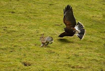
In this paper, the Harris hawks’ algorithm is used
to solve the following engineering problems. Figure 1 - Behavior of a Harris hawk during hun-ting
440 TEHNIKA – MAŠINSTVO 70 (2021) 4B. MILENKOVIĆ IMPLEMENTATION OF HARRIS HAWKS OPTIMIZATION (HHO)...
This algorithm consists of exploration phase, tra- perform a hard ( E 0.5 ) or soft ( E 0.5 )
nsition to exploitation phase, and exploitation phase.
besiege.
In the exploration phase, the hawks perch ran-
domly on some locations, waiting to detect the prey In the case of soft besiege, when r 0.5 and
(designated as „rabbit‟), which is the current best E 0.5 , the prey tries to escape the hawks, yet un-
solution, based on two strategies, each of which ha- successfully.
ving equal chance q to be selected. q is a random
variable having the value between 0 and 1, used for a This is modeled by the following equ-ations:
coin toss in this phase of the algorithm. If this va- X t 1 X t E JX rabbit t X t
riable’ s value is less than 0.5, the first strategy is ap- (3)
plied. Otherwise, the second strategy is applied. The
two fore mentioned strategies are: X t X rabbit X t (4)
X rand t r1 X rand t 2r2 X t , q 0.5 Where X t is the difference between the
X t 1
X rabbit t X m t r3 LB r4 UB LB , q 0.5 position vector of the rabbit and the current position
t Ј 2 1 r5 is the random jump strength of the
(1)
Where X t 1 is hawk position in iteration rabbit while trying to run away, and r5 is a random
t 1, X rand t is the position of a randomly selected variable inside (0,1).
hawk, X t is the hawk’s current position, X rabbit t In order to simulate the motion of the rabbit, the
value J changes randomly in each iteration.
is the current position of the rabbit, X m t is the
In the case of hard besiege, when r 0.5 and ,
current average position of the hawks. The constants
r1 , r2 , r3 , r4 are random number inside (0,1) which are E 0.5 the rabbit does not have enough energy to
updated in each iteration, while UB and LB represent escape, and the hawks move in for the attack. The
upper and lower bounds of variables. The first stra- positions in this case are updated using the following
tegy generates solutions based on a random position, equation:
and the current position of the selected hawk, while X t 1 X rabbit t E X t
the second strategy generates solutions based on (5)
current best solution, mean position of all hawks, and
the lower and upper bounds for each variable. In the case of soft besiege with progressive
rapid dives, when E 0.5 and r 0.5 , the rabbit
Based on escaping energy of the prey, this algo-
rithm switches between exploration and exploit-a- has enough energy to escape the attack, while the
tion phases. This energy is modeled as: hawks perform a soft besiege.
In order to model the movement of the esca-
t
E 2 E0 1 ping rabbit, the levy flight concept is used in this
T (2) algorithm. In order to per-form a soft besiege, the
hawks decide their next move based on equation:
where E indicates the escaping energy of the prey, T
is the maximum number of iterations, and E0 is the Y X rabbit t E JX rabbit t X t
(6)
initial state of its energy. When E 1 , this algorithm
This result is then compared to the previous dive,
is in exploration phase, while for E 1 , the algorithm to see if this dive will be good or not. If the dive is
is in exploitation phase. worse, the hawks perform random rapid dives when
In the exploitation phase, the hawks perform the approaching the rabbit, based on the following
surprise pounce described earlier, by attacking the equation:
intended prey. What can happen in this phase is that Z Y S x LF D (7)
the prey has enough energy to escape the dive,
meaning that the hawks will have to perform several where D is the dimension of problem and S is a
dives on it. This is modeled by the variable r, and the random vector by size 1x D and LF is the levy
prey has equal chances for escaping and not escaping
the dive. Whatever the prey does, the hawks will flight function, which is calculated using the follo-
wing equation:
TEHNIKA – MAŠINSTVO 70 (2021) 4 441B. MILENKOVIĆ IMPLEMENTATION OF HARRIS HAWKS OPTIMIZATION (HHO)...
1
using the formula for soft besiege
Г 1 x sin else if (r ≥0.5 and |E| < 0 . 5 ) then
u x 2
LF x 0.01 1 , 1
# hard besiege
1
Г 2 x x2 Update positions using the formula for hard besiege
2
(8) else if (r < 0 . 5 and |E|≥ 0 . 5 ) then
The constants u, are random values inside # soft besiege with progressive rapid dives
Update positions using the formula for soft besiege with
(0,1), while is the default constant set to 1.5. Based progressive rapid dives
on previous discussion, the final strategy for updating else if (r < 0 . 5 and |E| < 0 . 5 ) then
hawk position is given by: # hard besiege with progressive rapid dives
Y , if F Y F X t
Update positions using the formula for hard besiege with
X t 1 (9) progressive rapid dives
Z , if F Z F X t Return Xrabbit
In the case of hard besiege with progressive rapid 3. EXPERIMENTAL ENGINEERING EXAMPLES
dives, when E 0.5 i r 0.5 ,the rabbit does not FOR OPTIMIZATION
have enough energy to escape, and the hard besiege is In this section, for each of the optimization pro-
performed by the hawks. This time, the hawks try to blems we describe the basis of the problem, goal
decrease the distance to their average location with function, algorithm parameters, as well as conditions
the escaping prey. This is modeled by the following that are to be met. Every step of this process was done
equations: using the MATLAB R2019a software suite.
3.1. Optimization of the speed reducer
Y , if F Y F X t
X t 1 (10) The goal of speed reducer optimization is minimi-
Z , if F Z F X t zing the reducer weight whilst fulfilling all the de-
fined constraints.
Where Y and Z are given by the following In Figure 2 a schematic view of speed reducer is
equations: shown.
Y X rabbit t E JX rabbit t X m t
(11)
Z Y S x LF D (12)
The pseudocode for the algorithm is given below:
Pseudo-code of HHO algorithm
Inputs: The population size N and maximum number of
iterations T
Outputs: The location of rabbit and its fitness value
Initialize the random population Xi (i = 1 , 2 , . . . , N)
while (stopping condition is not met) do Figure 2 - Schematic view of the speed reducer with
Calculate the fitness values of hawks variable parameters
Set X rabbit as the location of rabbit (best location) Project variables for the speed reducer problem
for (each hawk (Xi )) do are: the width between the shafts (x1), the module of
Update the initial energy E0 and jump strength J the teeth (x2), the number of teeth in the pinion (x3),
E0 =2rand()-1, J=2(1-rand()) the length of the first shaft between the bearings (x4),
Update E the length of the second shaft between the bearings
if (|E|≥ 1) then (x5), the diameter of the first shaft (x6) and the dia-
# exploration phase meter of the second shaft (x7).
Update positions using the formula for Goal function to be minimized is defined as:
exploration phase
if (|E| < 1) then f x 0,7854 x1 x22 3,3333x32 14,933x3 43,0934 1,508x1 x62 x72
# exploitation phase 7,4777 x63 x73 0,7854 x4 x62 x5 x72
if (r ≥0.5 and |E|≥ 0 . 5 ) then (13)
# soft besiege Update positions Whilst the conditions to be met are:
442 TEHNIKA – MAŠINSTVO 70 (2021) 4B. MILENKOVIĆ IMPLEMENTATION OF HARRIS HAWKS OPTIMIZATION (HHO)...
27 the shell (x3) and thickness of the dish end (x4).Goal
g1 x 1 0 function to be minimized is defined as:
x1 x22 x3 (14)
f x 0,6224x1x3 x4 1,7781x2 x32 3,1661x12 x4 19,84x12 x3
397.5
g2 x 1 0 (26)
x1 x22 x32 (15) Whilst the conditions to be met are:
g3 x
1.93x53
1 0 g1 x x1 0,0193x3 0; (27)
x2 x3 x74
g2 x x2 0,00954 x3 0;
(16)
(28)
1.93x53
g4 x 1 0 4
x2 x3 x74 (17) g3 x x32 x4 x33 1296000 0;
3 (29)
1/2
475 x 2
4
16.9 10
6
g4 x x4 240 0;
x2 x3 (30)
g5 x 1 0
110 x63 (18) 0 xi 100; i 1, 2; (31)
1/2
475 x
10 xi 200; i 3, 4;
2
4
157.5 10
6
(32)
x2 x3
g6 x 1 0 3.3. Optimization of the cantilever beam
85 x73 (19)
In this part, we will be solving the popular stru-
x2 x3
g7 x 1 0 ctural design problem of a cantilever beam (Figure 4).
40 (20) The goal is to minimize the weight of the cantilever
beam.
5 x2
g8 x 1 0
x1 (21)
x1
g9 x 1 0
12 x2 (22)
15 x6 1.9
g10 x 1 0
x4 (23) Figure 4 - Schematic view of the speed cantilever
1.1x7 1.9 beam with variable parameters
g11 x 1 0
x5 As seen in Figure 4, the cantilever beam consists
(24)
of five hollow, box shaped bearings with a square
2,6 x1 3,6 ; 0,7 x2 0,8 ; 17 x3 28 shaped frame. Project variables are lengths of the five
7,3 x4 8,3 ; 7,3 x5 8,3 ; 2,9 x6 3,9 squares which make up the cantilever beam.
The goal function is defined by the equation:
5,0 x7 5,5 (25)
f x 0,6224 x1 x2 x3 x4 x5 ,
3.2. Optimization of the pressure vessel
(33)
Second problem is optimization of a pressure ve-
ssel (figure 3), which consists of reducing costs of Whilst the only constraint for this problem being:
material, montage and welding costs. 61 27 19 7 1
g x 1 0,
x13 x23 x33 x43 x53 (34)
0,01 x1 , x2 , x3 , x4 , x5 100,
(35)
3.4. Optimization of the tension/compression
Figure 3 - Schematic view of the speed pressure vessel
with variable parameters spring
Four variables are defined for this problem: radius In Figure 5, a schematic view of helical spring,
of the shell (x1), length of the shell (x2), thickness of along with all the project variables, is shown.
TEHNIKA – MAŠINSTVO 70 (2021) 4 443B. MILENKOVIĆ IMPLEMENTATION OF HARRIS HAWKS OPTIMIZATION (HHO)...
ant colony algorithm (MACA), grasshopper optimi-
zation algorithm (GOA), water cycle algorithm
(WCA), Ant Lion Optimization (ALO), and Method
of Moving Asymptotes (MMA), depending of
solutions found in literature.
A detailed display of the results obtained by HHO
Figure 5 - Schematic view of the spring with variable and a comparison with several results obtained by
parameters other methods, for the problem of speed reducer, are
This problem consists of three continual vaiables, shown in Table 1.
two linear constraints, and five nonlinear constraints, In the case of this problem, HHO has given better
given in inequality form. The goal of this optimization results than those found in literature.
is minimizing the weight of the spring.
For the pressure vessel problem, the expected
Goal function to be minimized is defined as: value for the goal function is 5885.3327, with the
results shown in Table 2.
f x x3 2 x2 x12
(36) Table 2. Comparison of results for the pressure vessel
Whilst the conditions to be met are: Variables MACA[9] GOA[10] WCA[11] HHO
3
xx
g1 x 1
x1 0.822 0.8736 0.7781 0.798
2 3
0; (37)
x2 0.406 0.4318 0.3846 0.393
71785 x14
x3 42.602 45.2666 40.3196 41.255
4 x22 x1 x2 1
g2 x
x4 170.484 199.9998 200 187.369
1 0;
12566 x2 x1 x1 5108 x1
3 4 2 f(x) 5964.50 7666.1258 5888.3327 5826.81
(38)
As in the case of the speed reducer problem, the
140, 45 x1 HHO algorithm gave better results than those found
g3 x 1 0; in literature. For the cantilever beam design problem,
x22 x3 (39) the results shown in Table 3, along with the results
x1 x2 obta-ined by ALO, MMA and GOA methods.
g4 x 0; (40)
1,5 Table 3. Comparison of results for the cantilever beam
0,05 x1 2; (41) Variables ALO[12] GOA[12] MMA[12] HHO
x1 6.018 6.011 6.010 6.011
0, 25 x2 1,3; (42) x2 5.311 5.312 5.300 5.349
2 x3 15; (43)
x3 4.488 4.483 4.490 4.476
x4 3.497 3.502 3.490 3.491
x5 2.158 2.163 2.150 2.145
4. RESULTS AND DISCUSSION
f(x) 1.339 1.339 1.340 1.34
In this section, the results obtained by using HHO In this case, the HHO gives the same result as the
algorithm on previously defined engineering pro-ble- MMA algorithm, while ALO and GOA gave better
ms is given. results.
Table 1. Comparison of results for the speed reducer Experimental research was performed for the
helical spring problem, and the results of HHO
Variables MACA[9] GOA[12] WCA[11] HHO
algorithm, along with the results for MACA, GOA,
x1 3.499 3.5 3.5 3.5 and WCA algorithms, are given in Table 4. The ex-
x2 0.699 0.7 0.7 0.7 pected value for the goal function in this case is
x3 17 17 17 17 0.012665.
x4 8.051 7.3 7.3 7.3 Table 4. Comparison of results for the spring
x5 8.084 7.8 7.715 7.8
x6 3.351 3.350 3.350 3.35021 Variables MACA[9] GOA[12] WCA[11] HHO
x7 5.286 5.287 5.286 5.28668 x1 0.0523 0.05 0.0516 0.0524
f(x) 3009.669 2996.964 2994.471 2995.542 x2 0.3722 0.3174 0.3562 0.3750
x3 10.4141 4.4584 11.3004 10.3038
Results of the Harris hawks’ algorithm (HHO)
will be compared to results obtained by the modified f(x) 0.0128 0.0128 0.0126 0.0126
444 TEHNIKA – MAŠINSTVO 70 (2021) 4B. MILENKOVIĆ IMPLEMENTATION OF HARRIS HAWKS OPTIMIZATION (HHO)...
In the case of helical spring optimization, HHO [2] Essam H. Houssein, Mosa e. Hosney, Mohamed
gives the same result as WCA, while MACA and Elhoseny, Diego Oliva, Waleed M. Mohamed, M.
GOA giving a slightly worse result. Hassaballah: Hybrid Harris hawks optimization
with cuckoo search for drug design and discovery in
5. CONCLUSION chemoinformatics, Scientific Reports, 10:14439,
2020.
Contemporary optimization entails applying mo-
dern optimization methods, particularly in the area of
[3] Saeid Khalifeh, Saeid Akbarifard, Vahid Khalifeh,
modern engineering, where in solving optimization
Ebrahim Zallaghi: Optimization of water
problems often means solving nonlinear goal functi- distribution of network systems using the Harris
ons with a large number of constraints and variables. Hawks optimization algorithm (Case study:
In order to solve optimization problems, one ne-eds to Homashahr city) MethodsX, Vol 7,2020,100948.
go through several steps.
Firstly, problem para-meters are to be identified. [4] Pei Du, Jianzhou Wang, Yan Hao, Tong Niu,
Secondly, the constraints for problem parameters Wendong Yang: A novel hybrid model based on
need be acknowledged. Thirdly, optimization pro- multi-objective Harris hawks optimization
blem goals must be resea-rched and considered thoro- algorithm for daily PM 2.5 and PM 10 forecasting,
ughly. Lastly, based on the identified parameters, Applied Soft Computing Journal, Vol 96, 2020,
constraints, and goal functions, a convenient optimi- 106620.
zation method must be chosen.
[5] Carlos A. Coello Coello: Constraint-handling inge-
This paper describes using Harris hawks’ optimi- netic algorithms through the use of dominance ba-
zation algorithm in order to solve a few engineering sed tournament selection, Advanced Engineering In-
problems with a constant number of variables. For formatics, 16, 193–203, 2002.
this algorithm, 50 search agents and 1000 iterations
were chosen as input parameters. [6] Sandgren E, Nonlinear integer and discrete progra-
During the course of the research, it has been mming in mechanical design optimization, Journal
noted that increasing sea-rch agent and iteration count of Mechanical Design;112(43):223-9, 1990.
did not yield better so-lutions. Therefore, this
combination of input para-meters was chosen, since it [7] A. Gandomi, X. S. Yang, A. H. Alavi, Cucko search
gives minimal execution time. algorithm:a metaheuristic approach to solve structural
optimization problems, Springer-Verlag, London,
In the case of speed reducer and pressure vessel
2011.
optimization, the Harris hawks’ algorithm gives better
results than other methods found in literature. The
[8] Arora J. S. Introduction to optimum design. New
results for the other two optimization problems, na-
York: McGraw-Hill; 1989.
mely the cantilever beam and helical spring problem,
were shown to be near optimal.
[9] S. Mirjalili, S. M. Mirjalili, A. Lewis, Grey wolf
This paper focuses on application of optimization optimizer, Advances in Engineering Software 69,
algorithms on engineering problems. In this field of 46-61, 2014.
study, further research is always necessary, due to its
applicability and possibility for the improvement of [10] Đ. Jovanović, B. Milenković, M. Krstić, Application
the optimization results. of Grasshopper Algorithm in Mechanical Engi-
neering, YOURS 2020, pp.1-6.
6. ACKNOWLEDGEMENT
This work was supported by the Serbian Ministry [11] H. Eskandar, A. Sadollah, A. Bahreininejad, M.
of Education, Science and Technological Develo- Hamdi: Water cycle algorithm – A novelmeta-heu-
pment through Mathematical Institute of the Serbian ristic optimization method for solving constrained
Academy of Sciences and Arts. engineering optimization problems, Computers and
Structures, 2012.
REFERENCES
[12] Shahrzad S, Seyedali Mirjalili and Andrew Lewis,
[1] Ali Asghar Heidari, Seyedali Mirjalili, Hossam Grasshopper Optimisation Algorithm: Theory and
Faris, Ibrahim Aljarah, Majdi Mafarja, Huiling Application, Advances in Engineering Software,
Chen: Harris hawks optimization: Algorithm and Volume105,March, pp.30-47, 2017.
applications, Future Generation Computer Systems,
March 2019. [13] https://en.wikipedia.org/wiki/Harris%27s_hawk
TEHNIKA – MAŠINSTVO 70 (2021) 4 445B. MILENKOVIĆ IMPLEMENTATION OF HARRIS HAWKS OPTIMIZATION (HHO)...
REZIME
IMPLEMENTACIJA ALGORITMA HARISOVOG JASTREBA ZA REŠAVANJE
INŽENJERSKIH PROBLEMA
U skorije vreme, tehnike optimizacije su postale veoma važne i popularne za primene u inženjerstvu. U
ovom radu je demonstriran Algoritam Harrisovog jastreba (Harris Hawks’ Optimization, HHO) za
rešavanje optimizacionih problema u inženjerstvu. U drugom delu rada, date su biološke osnove, kao i
objašenjenje principa rada algoritma. Nakon toga, HHO algoritam, kao i njegova primenjivost je
detaljno objašnjena. Pseudo kod je napisan u MATLAB R2019a softverskom paketu. HHO algoritam je
potom korišćen za rešavanje inženjerskih problema, poput: optimizacija reduktora, optimizacija suda
pod pritiskom, optimizacija konzolnog nosača, i optimizacija zategnute/sabijene opruge. Statistički re-
zultati, su pokazali da je HHO daje kompetitivno dobre rezultate, u poređenju sa drugim metaheuri-
stičkim algoritmima.
Ključne reči: algoritam Harisovog jastreba, optimizacija, inženjerski problemi, metaheuristike
446 TEHNIKA – MAŠINSTVO 70 (2021) 4You can also read