Design and Implementation of a New Algorithm for Enhancing MPPT Performance in Solar Cells - MDPI
←
→
Page content transcription
If your browser does not render page correctly, please read the page content below
Article
Design and Implementation of a New Algorithm for
Enhancing MPPT Performance in Solar Cells
Ehsan Norouzzadeh 1, Ahmad Ale Ahmad 2, Meysam Saeedian 3, Gholamreza Eini 4
and Edris Pouresmaeil 3,*
 1 Department of Electrical and Computer Engineering, Semnan University, Semnan 35131-19111, Iran;
   e.norouzzadeh@semnan.ac.ir
 2 Department of Electrical and Computer Engineering, Babol Noshirvani University of Technology,

   Babol 47148-71167, Iran; a.ahmad@nit.ac.ir
 3 Department of Electrical Engineering and Automation, Aalto University, 02150 Espoo, Finland;

   meysam.saeedian@aalto.fi
 4 Department of Electrical and Computer Engineering, Arak University of Technology, Arak 38181-41167,

   Iran; gholamrezaeini1371@gmail.com
 * Correspondence: edris.pouresmaeil@aalto.fi

 Received: 3 December 2018; Accepted: 30 January 2019; Published: 6 February 2019

 Abstract: This paper presents a new algorithm for improving the maximum power point tracking
 method in solar cells. The perturb and observe and the constant voltage algorithms are combined
 intelligently in order to have a fast response and a high power efficiency. Furthermore, a two-phase
 interleaved boost converter with a coupled inductor is used with the proposed algorithm. The
 input capacitor and inductor of this converter are much smaller than those of the conventional
 types of converters. Therefore, its inherent delay is too short. Computer simulations carried out in
 PowerSIM and experimental results using a 100 W prototype verify the superior performance of
 the proposed algorithm and converter. The operating principle and comparisons with the
 conventional algorithms and other methods are presented in this paper. Moreover, a cost function
 is presented to compare the new algorithm with the others. The experimental results show that the
 presented system tracks any changes in power in less than 10 ms, and a quick response to the
 maximum power point is achieved.

 Keywords: solar cells; maximum power point tracking; solar energy conversion

1. Introduction
     Fossil fuels are the major energy source that is declining over time and is also creating many
problems such as air pollution. Therefore, a great energy transition from fossil fuels to renewable
energy sources, particularly solar energy, is underway [1‒2]. Nonetheless, the efficiency of solar cells
(SCs) is low, and power delivery depends on ambient irradiation and temperature. Therefore, it is
necessary to extract the maximum available power from SC. There are several techniques to track the
maximum power point, which are known as maximum power point tracking algorithms.
     The perturb and observe (P&O) is the most popular maximum power point tracking (MPPT)
algorithm [3‒4]. In this algorithm, the output power is calculated in each cycle by sampling the
current and voltage of the SC. Then, according to the difference between the current output power
and the output power of the previous cycle, the operating point of the SC is modified to achieve the
maximum power point (MPP). Cheapness and low complexity are two advantages of using P&O. It
also does not depend on the characteristics of the SC. However, its response is slow and oscillates
around the MPP, especially when temperature or irradiation change extremely. An adaptive P&O
algorithm is suggested in Reference [5]. This algorithm consists of two parts: 1) the current

Energies 2019, 12, 519; doi:10.3390/en12030519                                www.mdpi.com/journal/energies
Energies 2019, 12, 519 2 of 17
perturbation algorithm and 2) the adaptive control algorithm. These two parts are based on the
conventional P&O and fractional short-circuit current algorithms. In References [6] and [7], a
modified P&O algorithm is used to improve the MPPT.
Another algorithm is the incremental conductance (IC) algorithm [4,8]. The IC algorithm is
based on the fact that the power slope of the SC at the MPP is zero (dP/dV = 0). In this algorithm,
incremental conductance (dI/dV) is compared with the instantaneous conductance (I/V) in each
cycle, and the operation point of the SC is moved to the MPP. The IC algorithm is similar to the P&O,
except that it presents better responses; however, its calculation is more complex. In Reference [9], a
novel variable step-size incremental-resistance MPPT algorithm is introduced, which atomically
adjusts the step size to track the MPP. This algorithm improves the steady-state and dynamic
response and has a wide operating range.
Constant voltage (CV) is an algorithm that is very simple to implement [10,11]. In the CV
algorithm, a fixed reference voltage (Vref) regulates the output voltage of the SC. The Vref is constant
and is extracted from the characteristics of the SC. Therefore, the operating point of the SC is always
kept near the MPP. A simple implementation and a fast response are the advantages of CV, but it
cannot find the exact MPP. In Reference [12], an adaptive voltage sensor is presented. This method
uses a variable scaling factor and a direct duty cycle control method, can determine the voltage by a
voltage divider circuit and can improve the transient and steady-state performance, without
employing a PI controller.
Fraction open-circuit voltage (VOC) is another MPPT algorithm [8]. In this algorithm, VMPP is
calculated as:
VMPP k VOC (1)
where k is usually between 0.7 and 0.9. This algorithm is simple, but its accuracy is low, and
determining best value of k is difficult. In Reference [13], a fuzzy agent adapted with the fractional
open-circuit voltage technique is used to track the MPP in a fast and accurate manner.
The reaction short-circuit current (ISC) algorithm is similar to the open-circuit algorithm [14]. In
this algorithm, the SC current is used to calculate the current at maximum power (IMPP) as follow:
I MPP k I SC (2)
This algorithm is more expensive than the fractional open-circuit voltage algorithm. In
Reference [13], a modified fractional short-circuit current MPPT algorithm is introduced on the basis
of the determination of the optimum slope of the power load line.
Moreover, some methods are based on a mathematical function. In Reference [14], a complex
function is introduced in order to track the maximum power point. The function is formed by a
two-dimensional Gaussian function and an arctangent function with an adaptive perturbation step
size. In Reference [15], a parameter-estimation-based MPPT method for the power of photovoltaic
generation, based on the measured voltages, currents, and the characteristics of the output function
of photovoltaic generation (PVG) is presented. The proposed MPPT method uses parameter
estimations to directly calculate the solar irradiance and temperature.
The neural network and the fuzzy logic controllers, which provide faster tracking of MPP and
present smoother signals with less fluctuation, are expensive and have high implementation
complexity [16,17]. In Reference [18], a new digital control scheme using a fuzzy-logic and a dual
MPPT controller is introduced. This paper employs the P&O algorithm, and in order to eliminate the
resulting state oscillations, the fuzzy logic controller is gradually updated. In Reference [19], to
decrease the energy loss in the MPPT circuit, a successive approximation register method that has a
power-down mode is proposed, based on a hill climbing algorithm with a fast-tracking time. This
MPPT technique specifies the direction of the perturbation and employs the binary search method of
the successive approximation.
Besides the methods mentioned above, many other methods are employed. In Reference [20], a
new method of tracking the MPP of a photovoltaic module is presented, which exploits the effects of
the inherent characteristic resistances of the PV cells. An analysis of the IV characteristics of the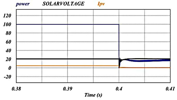
Energies 2019, 12, 519 3 of 17
photovoltaic module in the IV plane revealed the possibility of predicting the MPP by finding the
maximum possible power rectangle within an analysis of the IV characteristics. In Reference [21], a
robust input–output linearization controller that establishes a linear mapping between the duty
cycle and the SC voltage is proposed. This method consists of a dynamic assignment and linearizing
control. In Reference [22], to improve time tracking and MPPT efficiency, an adaptively
binary-weighted step and a monotonically decreased step are used.
This paper proposes a new MPPT algorithm in order to obtain a fast and accurate response in
solar cells. The new algorithm is an intelligent combination of the P&O and the CV algorithms
(CPV). When the irradiation changes suddenly, the operation point gets close to the MPP using the
CV algorithm. Then, the P&O algorithm will find the new MPP, exactly. A two-phase interleaved
boost converter with a coupled inductor is used because of its much greater reduction of the input
switching current ripple. Therefore, an interleaved boost converter (IBC) does not need a bulk input
capacitor. The successful performance of the MPPT algorithm is verified through a simulation and
the related experimental results.
2. Solar Cell
SCs are electrical devices that convert the sun’s energy directly into electricity, when exposed to
sunlight. A SC is a positive- negative (PN) junction with a large surface area which allows light to
pass through the PN junction. Thus, its mathematical equation is represented by [23]:
I D I rs e qV / kT 1 I L (3)
where ID is the diode current (A), IL is the light generated current (A), Irs is the diode saturation
current (A), q is the electron charge (1.6 × 10⁻¹⁹ C), k is the Boltzmann constant (1.38 × 10⁻²³ J/K), and T
is the cell temperature (K). This equation can be considered as having two parts: the current
described by the usual diode equation and the current due to the light generation. The power
delivered from the diode and solar energy is then converted into electricity when the diode begins to
shift down into the fourth quadrant. The physical model of a solar cell including the current source,
diode, and parallel and series resistance is shown in Figure 1.
Rs I
IL Rsh V
Figure 1. Physical model of the solar cell (SC).
The basic equation describing the model of a solar cell is as follows [3,16]:
q (V IRs )
KT
V IRs
I I L I rs (e 1) (4)
Rsh
where (V) and (I) are the cell voltage (V) and the current (A), respectively. (Rs) is the equivalent series
resistance, and (Rsh) shows the parallel resistance. The ‘I–V’ characteristic of a typical SC is shown in
Figure 2a.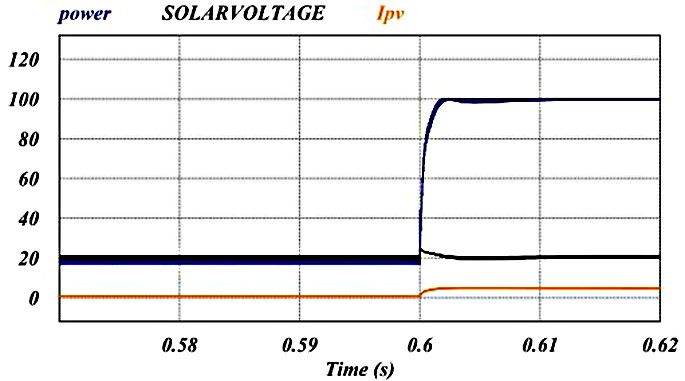
Energies 2019, 12, 519                                                                                               4 of 17

                              (a)                                                    (b)
      Figure 2. SC current versus voltage characteristic; (a) is the actual curve, (b) is the approximate curve.

3. Proposed MPPT Algorithm

3.1. CPV Algorithm
      The P&O and the CV algorithms are two popular MPPT algorithms because of their simplicity,
cheapness, and independence from the environmental conditions. The response of the P&O
algorithm is very slow, but the exact MPP can be found, and the output power ripple is very small
around the MPP. On the other hand, the CV response is fast, but it can only keep the operation point
near the MPP. Figure 3a,b show the P&O and CV algorithm performances for different irradiation
levels, respectively. Let us assume that the SC is at point A (MPP of curve 1) and that suddenly the
irradiation reduces to curve 2. If the P&O algorithm is used, the operation point reaches the point C,
far from the MPP of curve 2. Then, the P&O algorithm will move slowly to the operation point to B
(MPP of curve 2). In addition, the return trajectory is B→D→A when the irradiation increases to
curve 1. In the CV algorithm, when the irradiation reduces to curve 2, the operation point reaches
point E. E is not the MPP at the new irradiation but it is close to point B (MPP of curve 2), as shown
in Figure 3b.

                                                       A                                                         A
             Power (W)

                                                                           Power (W)

                         1                                     D                           1
                                                   B                                                         B
                         2   C                                                             2                     E

                              Voltage (V)                                                      Voltage (V)

                                 (a)                                                               (b)

                                                                                       A
                                                                            F
                                       Power (W)

                                                           1

                                                           2                  B
                                                                                       E

                                                                   Voltage (V)

                                                                     (c)
      Figure 3. Maximum power point tracking by using (a) the perturb and observe (P&O) algorithm, (b)
      the constant voltage (CV) algorithm, (c) the proposed algorithm.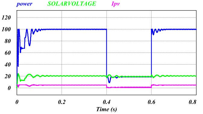
Energies 2019, 12, 519 5 of 17
The proposed algorithm uses both the P&O and the CV algorithms. Figure 3c shows the
trajectory of the SC operation point under the proposed algorithm. In this algorithm, when the
irradiation changes suddenly, the operation point gets rapidly closer to the MPP by the CV
algorithm. Then, P&O will find exactly where the new MPP is. Figure 4 shows the flowchart of the
proposed algorithm. According to Figure 4, if the irradiation changes strongly and ΔP is larger than
ΔPmax, then Vref will stay fixed, otherwise the P&O will not perform reliably. In the proposed
algorithm, the selection of ΔPmax is an important issue. It depends on the characteristics of the SC and
the weather conditions. However, a good selection will be as follows:
ΔPmax 0.04 maximum power of SC (5)
Start
V(k-1)=V(k)
P(k-1)=P(k)
Measure VPV, IPV
PPV(k)=VPV(k)*IPV(k)
Yes
ΔP=0
No
|ΔP|>ΔPmax Yes ΔV=0 Vref(k)=Vref(k-1)
No
No Yes
ΔP>0
No Yes Yes No
dv>0 dv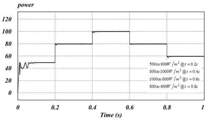
Energies 2019, 12, 519 6 of 17
Substituting Equations (6) and (7) into Equation (8) gives the following:
2 2
ΔP V2m(V2 VOC ) Vm
1 (V1 VOC ) = mV2 mV2VOC mV1 mVV ( 22 V12 ) mVOC (V1 V2 )
1 OC mV (10)
Equation (10) can be rearranged as follows:
ΔP m(V2 V1 )(V2 V1 ) mVOC (V1 V2 ) (11)
The voltage difference ΔV is defined as
ΔV V2 V1 (12)
Thus, substituting Equation (10) into Equation (9) gives
ΔP V (m(V2 V1 VOC )) (13)
Since V1 and V2 are smaller than Voc:
ΔP ΔV mVOC (14)
Therefore, Equation (14) can be written in the following form:
ΔP
ΔV (15)
m VOC
Therefore, the relation between ΔP and ΔV can be obtained from Equation (15).
3.3. Boost Converter
As shown in Figure 5, a boost converter is usually used for solar systems because of the
continuous input current. However, it suffers from the inherent switching ripple. In a conventional
boost converter, the input current ripple is between 30 to 60% of the nominal input current, as shown
in Figure 6. This ripple causes a large power ripple in solar cells, which is unfavorable for solar
systems.
As shown in Figure 7, to resolve this problem, a very bulk electrolyte capacitor or inductor is
often connected to the input of boost converter. This solution increases the inherent delay of the
boost converter, because they are energy-storage elements. While the response time of a boost
converter is slow, it cannot be expected from the MPPT algorithm to have a fast response. In
addition, there is a limitation on the lifespan of the bulk electrolyte capacitor.
L
SW
Load
SC
Cin Cout
PWM
PI
V PV
V ref
MPPT +
-
I PV
V PV
Figure 5. SC system configuration (PWM: pulse width modulation, PI: proportional–integral
controller, SW: switch).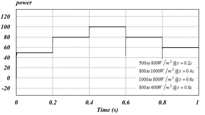
Energies 2019, 12, 519                                                                                    7 of 17

                                           Ib

                                                                       t
                                                Ts=1/fs

           Figure 6. Input current ripple of a non-isolated boost converter in continuous current mode.

                                                                                     Load
                           SC

                                   Figure 7. SC with an added input capacitor

      Another solution to reduce the input current ripple is using an interleaved boost converter
(IBC). The n-phase interleaved boost converters are driven at 360/n degrees out of phases. Thus, the
input effective switching current ripple is very largely reduced, because the n-phases are combined
together. Therefore, an IBC does not need a bulk input capacitor. An IBC can improve the conversion
efficiency and minimize switching losses, too. Thus, the IBC overcomes the drawbacks of the
conventional boost converter.
      In the proposed method, a two-phase interleaved boost converter with coupled inductor was
employed. The coupled inductor distributed the input current equally, and the inherent current was
not returned. The IBC is shown in Figure 8.

                                    V PV
                                                   V ref

                                   I PV

                                                           V PV

      Figure 8. Block diagram of the interleaved boost converter (IBC) used in the proposed method for the
      SC system.

4. Analysis of the Simulation and Experimental Results
     The proposed algorithm and the IBC were verified by a simulation and related experimental
results from a 100 W prototype. The solar cell and boost converter parameters are listed in Tables 1
and 2.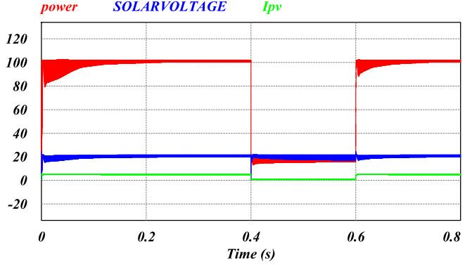
Energies 2019, 12, 519                                                                                               8 of 17

                                         Table 1. Characteristics of the 100 W solar cell.

                             Symbol                         Quantity                              Value
                              PMPP                      Maximum power                            100 W
                              VMPP                 Voltage at maximum power                      20.45 V
                              IMPP                 Current at maximum power                      4.89 A
                              VOC                      Open circuit voltage                       25 V
                               ISC                     Short circuit current                     5.19 A
                           αISC (%/0C)            Current temperature coefficient                 0.024
                          βVOC (%/0C)             Voltage temperature coefficient                −0.356

                                          Table 2. Specification of the boost converter.

                                       Symbol           Quantity                       Value
                                         Vin          Input voltage                   15‒25 V
                                         Vout        Output voltage                   26‒30 V
                                         Imax     Maximum input current                 6A
                                          fsw      Switching frequency                12 KHz
                                         Cin         Input capacitor                    1 uF
                                           L           Inductance                     370 uH
                                          M         Mutual inductance                 300 uH

     In some references, a resistance has been chosen as a load for boost converters, but this is not
correct for the boost converter used in the solar cell system [5,9,12,14,24,25]. In this system, the boost
converter runs the MPPT algorithm, and its output voltage cannot be regulated. Therefore, the load
should regulate the output voltage with the absorbing power from the DC link. In a real solar cell
system, an inverter or battery bank, which are connected to the output of the solar converter, do this
task properly. To simulate the behavior of the inverter or battery bank, a voltage-controlled current
source was used as the load of the boost converter. Figure 9a shows the block diagram of the load,
and the circuit of the voltage-controlled current source is shown in Figure 9b.
     The maximum power consumption of the load was 100 W and it adjusted the DC link voltage
around 26 V.

                                                                                                                     Vin
    DC link
                                                       R6
                                                                                          Vcc                   R7
                                                                                  +
                                                                 Vcc
                                                                                  -
                                                      RP                                              R4   R5
                                                               R3
                               +
                                   -       PI
                                                                       R1    R2       C

                         (a)                                                               (b)
      Figure 9. (a) Block diagram of the voltage-controlled current source, (b) circuit of the
      voltage-controlled current source.

    Table 3 shows the MPPT algorithm parameters. To reduce the power oscillation to less than 0.1
W around the MPP, ΔV was calculated and resulted to be 4 mV according to Equation (14).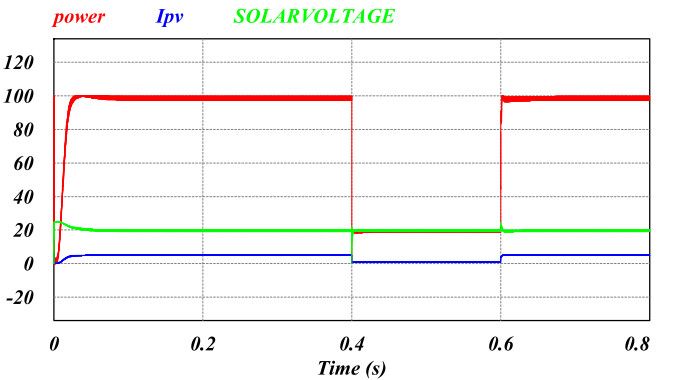
Energies 2019, 12, 519                                                                            9 of 17

                   Table 3. Parameters of the maximum power point tracking (MPPT) algorithm.

                                             Parameter      Value
                                               ΔPmax         4W
                                                ΔP          0.1 W
                                                ΔV          4 mV

4.1. Simulation Results and Analysis
      The proposed MPPT algorithm was simulated in powersim (PSIM) for a 100 W solar cell. In the
simulation, the performance of the system was studied at the sudden change of irradiation. It was
assumed that the irradiation suddenly decreased from 1000 W/m2 to 200 W/m2 at 0.4 s and then
increased to 1000 W/m2 at 0.6 s. Figure 10 shows the simulation results. According to Figures 10b and
10c, the system tracked and found the MPP properly in and less than 2 ms. In addition, the MPPT
efficiency was more than 99%.

                                                      (a)

                                                     (b)

                                                      (c)
      Figure 10. (a) Simulation results of power, voltage, and current with irradiation changes, (b)
      decreasing the irradiation, (c) increasing the irradiation.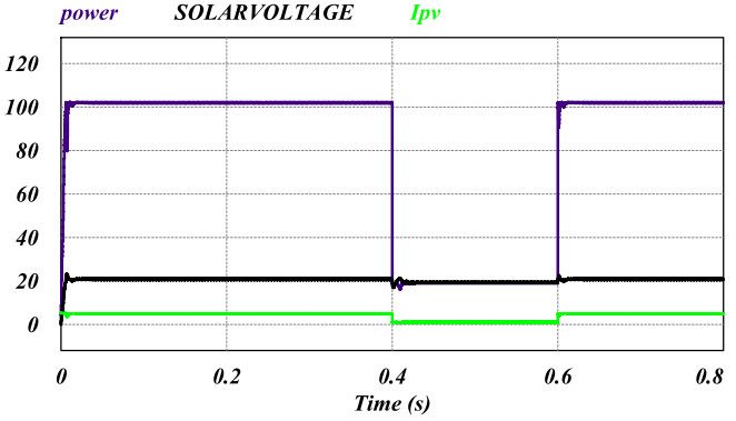
Energies 2019, 12, 519 10 of 17
4.2. Experimental Results and Analysis
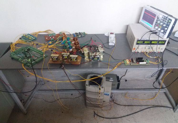
To verify the performance of the new algorithm and the proposed converter, a 100 W prototype
was implemented. The control unit of the system was implemented by a digital signal processor
(DSP) TMS320F28335.
Because of the laboratory limitation, the solar irradiation was simulated by 12 incandescent
lamps (220 V, 200 W). Figure 11 shows the solar cell prototype. The experimental results are shown
in Figure 12, and the waveforms of power, voltage, and current are illustrated when the irradiation
suddenly changed from the maximum to the minimum available irradiation and vice versa. The
maximum and the minimum irradiation were 400 W/m2 and 70 W/m2, respectively. According to
Figure 12, the proposed algorithm tracking time was less than 4 ms and the system could find the
MPP properly.
Figure 11. The implemented SC system in the laboratory.Energies 2019, 12, 519 11 of 17
Figure 12. Experimental results with irradiation changes by the proposed algorithm (a) power, (b)
current, (c) voltage, (d) reference voltage, (e) power by the P&O algorithm.
4.3. Comparative Study
To study the suitable performance of the proposed algorithm, the results were compared with
those from the conventional algorithms. To compare in the same conditions, a cost function (CF) was
defined for the converter. The cost function is the ratio of the energy stored in the converter to the
maximum energy produced by the solar cell. The cost function is given as:
Cin V 2 +LI 2
CF f sw (16)
Pmax
where Pmax is the maximum power of the solar cell (W), Cin is the input capacitor (µF), V is the
MPP voltage over the input capacitor (V), L is the inductor (mH), I is the current flows in the
inductor at maximum power (A), and fsw is the switching frequency (kHz).
The MPPT efficiency, tracking time, and cost function are presented in Table 4 for the proposed
MPPT algorithm, conventional P&O and IC algorithms, and other references. It should be noted
that, in this paper, the irradiation condition was worse than in other papers.
Table 4. The comparison between the proposed algorithm, conventional algorithms, and validated
papers.
Time Tracking
Algorithm MPPT Efficiency Cost Function
Decreasing Irradiation Increasing Irradiation
P&O 0.45 s 0.72 s 99% 29.87
IC 0.5 s 0.9 s 98% 164
[5] 0.36 s 0.82 s 99% 29.87
[9] 0.15 s 0.15 s 99% 164
[12] 0.25 s 0.25 s 99% -
[24] 0.12 s 0.06 s 99% 29.87
[25] 0.05 s 0.05 s 99% -
Proposed (CPV) 0.002 s 0.002 s 99% 2.17
According to Table 4, the time tracking of the proposed algorithm was at least 30 times less than
in other papers, while the MPPT efficiency was 99%. According to the reform model, the cost
function was at least 7 times less than in other papers. This shows that the volume of the passive
elements of the proposed converter were 15 times smaller than in other studies.
Some simulation results with more details are presented below, based on architecture and on
the proposed algorithm.
It was assumed that the irradiation decreased from 1000 W/m2 to 200 W/m2 at 0.4 s and then
increased to 1000 W/m2 at 0.6 s again. Figure 13 shows the simulation results under the proposed
algorithm, combining the P&O and the CV algorithms, and the MPPT efficiency and tracking time
are presented in Table 5.Energies 2019, 12, 519 12 of 17
(a)
(b)
(c)
Figure 13. Simulation results of the power, voltage, and current under irradiation changes with (a)
the proposed algorithm, (b) the P&O algorithm, and (c) the CV algorithm.
According to Table 1, time tracking and MPPT efficiency were improved with the proposed
algorithm.
Table 5. The comparison between the proposed algorithm, the conventional algorithm, and the CV
algorithm in terms of time tracking and efficiency.
Time Tracking
Algorithm MPPT Efficiency
Decreasing Irradiation Increasing Irradiation
P&O 0.02s 0.032s 98%
CV 0.002s 0.002s 95%
Proposed (CPV) 0.002s 0.0024s 99%
As shown in Figure 14, another irradiation condition was tested. It was assumed that the
irradiation increased from 500 W/m2 to 800 W/m2 at 0.2 s and then increased to 1000 W/m2 at 0.4 s.
Afterwards, it decreased from 1000 W/m2 to 800 W/m2 at 0.6 s and from 800 W/m2 to 600 W/m2 at 0.8
s. As shown in Figure 14, the proposed algorithm was better than the conventional algorithm;
therefore, the proposed algorithm has a fast speed and high efficiency under these conditions.Energies 2019, 12, 519 13 of 17
(a)
(b)
(c)
Figure 14. Simulation results of the power changes under irradiation changes with (a) the proposed
algorithm (b), the P&O algorithm, (c) the CV algorithm.
More irradiation levels are considered in Figure 15, in which output power under the proposed
method and the P&O and CV algorithms are reported:
(a)Energies 2019, 12, 519 14 of 17
(b)
(c)
Figure 15. Simulation result of the power changes under irradiation changes with (a) the proposed
algorithm, (b) the P&O algorithm, (c) the CV algorithm.
As shown in Figure 15, at the abrupt irradiation levels, the proposed algorithm tracked the MPP
with high speed and high efficiency, but both the P&O and the CV algorithms did not have high
performance.
As we discussed in the paper, choosing the appropriate structure leads to a lower cost function
and does not require a bulk capacitor. However, high-speed tracking and high-MPPT efficiency are
impossible by a conventional boost converter. In order to verify the performance of this type of
converter, it was compared with a conventional converter with the same proposed algorithm.
(a)Energies 2019, 12, 519 15 of 17
(b)
Figure 16. Simulation results of the power changes under irradiation changes with (a) the IBC
converter, (b) a conventional converter.
It was assumed that the irradiation decreased from 1000 W/m2 to 200 W/m2 at 0.4 s and again
increased to 1000 W/m2 at 0.6 s. Figure 16a shows the simulation results with a selective converter,
and Figure 16b shows the simulation results with a conventional boost converter. The MPPT
efficiency and tracking time are presented in Table 2 for the proposed MPPT, the conventional P&O,
and the CV. The comparative results are shown in Table 2.
Table 6. The comparison between a conventional and the interleaved boost converter (IBC) on the
basis of the proposed algorithm.
Time Tracking
Converter MPPT Efficiency
Decreasing Irradiation Increasing Irradiation
Conventional 0.002 s 0.002 s 99%
IBC 0.002 s 0.002 s 99%
According to Table 6, the results obtained by a conventional converter were the same with the
selected structure if the input capacitor in the conventional boost converter was equal to 1000 uF,
while the input capacitor in the selected converter was equal to 1 uF. Figure 17 was obtained by
considering a conventional boost converter with a cost function equal to 2. As shown in this figure, it
had a low performance (i.e., time tracking was 0.004 s, and efficiency was 91%).
Figure 17. Simulation results of the power changes under irradiation changes with (a) the proposed
algorithm, (b) the P&O algorithm.
Consequently, the proposed structure was effective for practical MPPT.
5. Conclusions
In this paper, the popular P&O and CV algorithms were used to obtain a fast response and a
high MPPT efficiency. In the proposed algorithm, the CV algorithm regulates the operation point of
the solar cell around the MPP when irradiation changes suddenly. Then, the P&O algorithm finds
the exact MPP. Therefore, the new algorithm is an intelligent combination of the P&O and the CV
algorithms. The simulation results of the 100 W prototype verified the performance of the proposed
algorithm. The boost converter of the prototype was redesigned. It is a two-phase interleaved boost
converter with a coupled inductor, which improved the conversion efficiency and minimized
switching losses and the inherent switching ripple. To simulate the behavior of the inverter or
battery bank, a voltage-controlled current source was used as the load of the boost converter. The
experimental results showed that the tracking time was less than 2 ms, which is at least 30 times
better than the time required by other conventional algorithms. In addition, a cost function (CF) was
defined for the converter to compare the proposed method with other methods. The results showedEnergies 2019, 12, 519 16 of 17
that the cost function was about seven times lower than with other methods. Therefore, the volume
of the passive elements was 15 times smaller than in other studies.
Author Contributions: All authors contributed equally to this work and all authors have read and approved
the final manuscript.
Funding: This research received no external funding.
Conflicts of Interest: The authors declare no conflicts of interest.
References
1. Rahmanian, E.; Akbari, H.; Sheisi, G.H. Maximum power point tracking in grid connected wind plant by
using intelligent controller and switched reluctance generator. IEEE Trans. Sustain. Energy 2017, 8, 1313–
1320, doi:10.1109/TSTE.2017.2678679.
2. De Brito, M.A.G.; Galotto, L.; Sampaio, L.P.; e Melo, G.D.A.; Canesin, C.A. Evaluation of the main mppt
techniques for photovoltaic applications. IEEE Trans. Ind. Electron. 2013, 60, 1156–1167,
doi:10.1109/TIE.2012.2198036.
3. Femia, N.; Petrone, G.; Spagnuolo, G.; Vitelli, M. Optimization of perturb and observe maximum power
point tracking method. IEEE Trans. Power Electron. 2005, 20, 963–973, doi:10.1109/TPEL.2005.850975.
4. Sera, D.; Mathe, L.; Kerekes, T.; Spataru, S.V.; Teodorescu, R. On the perturb-and-observe and incremental
conductance mppt methods for pv systems. IEEE J. Photovolt. 2013, 3, 1070–1078,
doi:10.1109/JPHOTOV.2013.2261118.
5. Kollimalla, S.K.; Mishra, M.K. A Novel Adaptive P&O MPPT Algorithm Considering Sudden Changes in
the Irradiance. IEEE Trans. Energy Convers. 2014, 29, 602–610, doi:10.1109/TEC.2014.2320930.
6. Ahmed, J.; Salam, Z. A modified p&o maximum power point tracking method with reduced steady-state
oscillation and improved tracking efficiency. IEEE Trans. Sustain. Energy 2016, 7, 1506–1515,
doi:10.1109/TSTE.2016.2568043.
7. Macaulay, J.; Zhou, Z. A Fuzzy Logical-Based Variable Step Size P&O MPPT Algorithm for Photovoltaic
System. Energies 2018, 11, 1340, doi:10.3390/en11061340.
8. Esram, T.; Chapman, P.L. Comparison of photovoltaic array maximum power point tracking techniques.
IEEE Trans. Energy Convers. 2007, 22, 439–449, doi:10.1109/TEC.2006.874230.
9. Mei, Q.; Shan, M.; Liu, L.; Guerrero, J.M. A novel improved variable step-size incremental-resistance mppt
method for pv systems. IEEE Trans. Ind. Electron. 2011, 58, 2427–2434, doi:10.1109/TIE.2010.2064275.
10. Faranda, R.; Leva, S. Energy comparison of mppt techniques for pv systems. WSEAS Trans. Power Syst.
2008, 3, 446–455.
11. Dallago, E.; Liberale, A.; Miotti, D.; Venchi, G. Direct mppt algorithm for pv sources with only voltage
measurements. IEEE Trans. Power Electron. 2015, 30, 6742–6750, doi:10.1109/TPEL.2015.2389194.
12. Killi, M.; Samanta, S. An adaptive voltage-sensor-based mppt for photovoltaic systems with sepic
converter including steady-state and drift analysis. IEEE Trans. Ind. Electron. 2015, 62, 7609–7619,
doi:10.1109/TIE.2015.2458298.
13. Adly, M.; El-Sherif, H.; Ibrahim, M. Maximum power point tracker for a pv cell using a fuzzy agent
adapted by the fractional open circuit voltage technique. In Proceedings of the IEEE International
Conference in Fuzzy Systems (FUZZ), Taipei, Taiwan, 27–30 June 2011; pp. 1918–1922.
14. Tousi, S.R.; Moradi, M.H.; Basir, N.S.; Nemati, M. A function-based maximum power point tracking
method for photovoltaic systems. IEEE Trans. Power Electron. 2016, 31, 2120–2128,
doi:10.1109/TPEL.2015.2426652.
15. Teng, J.H.; Huang, W.H.; Hsu, T.A.; Wang, C.Y. Novel and fast maximum power point tracking for
photovoltaic generation. IEEE Trans. Ind. Electron. 2016, 63, 4955–4966, doi:10.1109/TIE.2016.2551678.
16. Manuel Godinho Rodrigues, E.; Godina, R.; Marzband, M.; Pouresmaeil, E. Simulation and Comparison of
Mathematical Models of PV Cells with Growing Levels of Complexity. Energies 2018, 11, 2902,
doi:10.3390/en11112902.
17. Kumar, K.K.; Bhaskar, R.; Koti, H. Implementation of mppt algorithm for solar photovoltaic cell by
comparing short-circuit method and incremental conductance method. Procedia Technol. 2014, 12, 705–715,
doi:10.1016/j.protcy.2013.12.553.
18. Al Nabulsi, A.; Dhaouadi, R. Efficiency optimization of a dsp-based standalone pv system using fuzzy
logic and dual-mppt control. IEEE Trans. Ind. Inform. 2012, 8, 573–584, doi:10.1109/TII.2012.2192282.Energies 2019, 12, 519 17 of 17
19. Kim, H.; Kim, S.; Kwon, C.K.; Min, Y.J.; Kim, C.; Kim, S.W. An energy-efficient fast maximum power point
tracking circuit in an 800-µw photovoltaic energy harvester. IEEE Trans. Power Electron. 2013, 28, 2927–
2935, doi:10.1109/TPEL.2012.2220983.
20. Raj, J.C.M; Jeyakumar, A.E. A novel maximum power point tracking technique for photovoltaic module
based on power plane analysis of I–V characteristics. IEEE Trans. Ind. Electron. 2014, 61, 4734–4745,
doi: 10.1109/TIE.2013.2290776.
21. Espinoza-Trejo, D.R.; Bárcenas-Bárcenas, E.; Campos-Delgado, D.U.; De Angelo, C.H. Voltage-oriented
input–output linearization controller as maximum power point tracking technique for photovoltaic
systems. IEEE Trans. Ind. Electron. 2015, 62, 3499–3507, doi:10.1109/TIE.2014.2369456.
22. Hong, Y.; Pham, S.N.; Yoo, T.; Chae, K.; Baek, K.H.; Kim, Y.S. Efficient maximum power point tracking for
a distributed pv system under rapidly changing environmental conditions. IEEE Trans. Power Electron.
2015, 30, 4209–4218, doi:10.1109/TPEL.2014.2352314.
23. Streetman, B.G. Solid State Electronic Devices; Prentice Hall: Upper Saddle River, NJ, USA, 2005.
24. Kollimalla, S.K.; Mishra, M.K. Variable perturbation size adaptive p&o mppt algorithm for sudden
changes in irradiance. IEEE Trans. Sustain. Energy 2014, 5, 718–728, doi:10.1109/TSTE.2014.2300162.
25. Moo, C.S.; Wu, G.B. Maximum power point tracking with ripple current orientation for photovoltaic
applications. IEEE J. Emerg. Sel. Top. Power Electron. 2014, 2, 842–848, doi:10.1109/JESTPE.2014.2328577.
© 2019 by the authors. Licensee MDPI, Basel, Switzerland. This article is an open
access article distributed under the terms and conditions of the Creative Commons
Attribution (CC BY) license (http://creativecommons.org/licenses/by/4.0/).You can also read