Barriers to Technology Adoption: What We Know from Micro Empirics Lauren Falcao Bergquist April 1, 2021
←
→
Page content transcription
If your browser does not render page correctly, please read the page content below
Barriers to Technology Adoption:
                     What We Know from Micro Empirics

                          Lauren Falcao Bergquist

                         STEG Macro Development Course

                                April 1, 2021

Bergquist (U Mich)             STEG Macro Development    April 1, 2021   1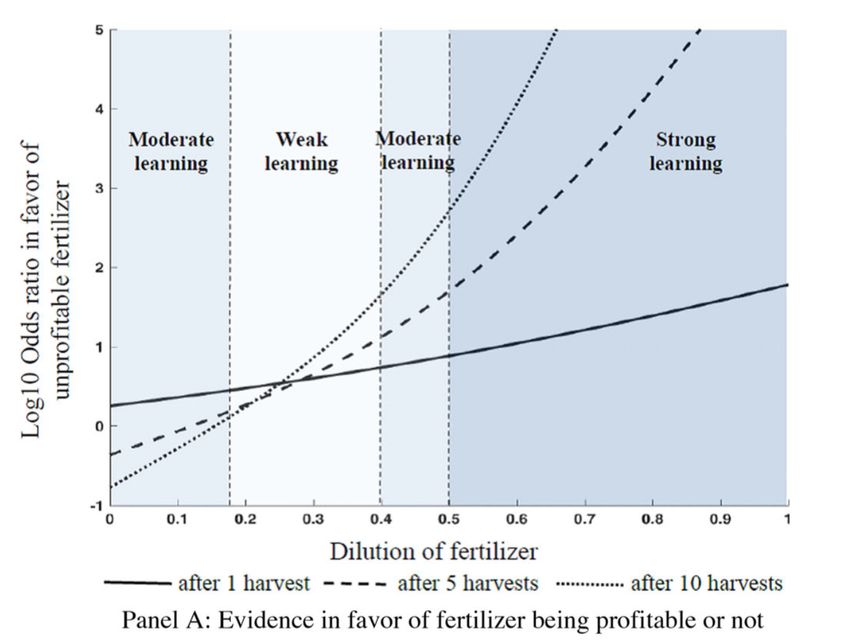
Big picture for this lecture
    Why are we talking about micro evidence in a class on macro topics?

    Bergquist (U Mich)      STEG Macro Development      April 1, 2021     2
Big picture for this lecture
    Why are we talking about micro evidence in a class on macro topics?
       1   Ag tech adoption is an area in which we have a large amount of
           well-identified estimates on constraints at the micro level = fodder for
           new macro models

       2   Limits to what can be studied by micro approaches alone

    Bergquist (U Mich)           STEG Macro Development          April 1, 2021        2
Big picture for this lecture
    Why are we talking about micro evidence in a class on macro topics?
       1   Ag tech adoption is an area in which we have a large amount of
           well-identified estimates on constraints at the micro level = fodder for
           new macro models

       2   Limits to what can be studied by micro approaches alone

    Goals for today’s class:
       1   Review (some of) the extensive micro literature on agricultural
           technology adoption

       2   Highlight ways that macro and micro can speak to, build off each other
           more in this area

    Bergquist (U Mich)           STEG Macro Development          April 1, 2021        2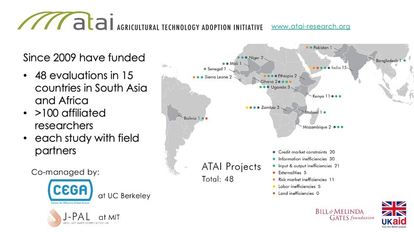
Big picture for this lecture
    Why are we talking about micro evidence in a class on macro topics?
       1   Ag tech adoption is an area in which we have a large amount of
           well-identified estimates on constraints at the micro level = fodder for
           new macro models

       2   Limits to what can be studied by micro approaches alone

    Goals for today’s class:
       1   Review (some of) the extensive micro literature on agricultural
           technology adoption

       2   Highlight ways that macro and micro can speak to, build off each other
           more in this area

    Goals for TA section next week (Eleanor Wiseman)
       1   Review emerging evidence on intermediation in agriculture (new, ripe
           area for micro/macro interaction)
    Bergquist (U Mich)           STEG Macro Development          April 1, 2021        2
Agricultural technology adoption
Agriculture has a key role in the economy of many developing
countries
Low productivity. Agriculture is:
64% of labor force but only 34% of GDP in SSA (2008)
43% of labor force but only 20% of GDP in Asia (2008)
2% of labor force and 2% of GDP in U.S.
Lack of technology adoption (e.g. input usage) plays a key role in
shaping these patterns
True in many regions, especially in SSA
Bergquist (U Mich) STEG Macro Development April 1, 2021 3Technology adoption Green Revolution technologies: high-yielding varieties of cereals, fertilizers, insecticides and pesticides, and irrigation Bergquist (U Mich) STEG Macro Development April 1, 2021 4
Technology adoption

   Green Revolution technologies: high-yielding varieties of cereals,
   fertilizers, insecticides and pesticides, and irrigation
   Increased production worldwide, particularly in developing countries
   (Gollin et al, 2021)
          Credited with saving over a billion people from starvation
          Norman Borlaug, the “Father of the Green Revolution,” received the
          Nobel Peace Prize in 1970s

   Bergquist (U Mich)          STEG Macro Development        April 1, 2021     4
Technology adoption
Green Revolution technologies: high-yielding varieties of cereals,
fertilizers, insecticides and pesticides, and irrigation
Increased production worldwide, particularly in developing countries
(Gollin et al, 2021)
Credited with saving over a billion people from starvation
Norman Borlaug, the “Father of the Green Revolution,” received the
Nobel Peace Prize in 1970s
But the Green Revolution did not transform agricultural productivity
everywhere
CGAP 2016 using FAO data; Infographic Data Source: World Development Indicators, FAO via the World Bank
Bergquist (U Mich) STEG Macro Development April 1, 2021 4Yields and fertilizer use
Bergquist (U Mich) STEG Macro Development April 1, 2021 5Adoption and market inefficiencies
Some technologies not adopted because they are not profitable
Increase in yields, but even more in costs (esp. labor)
Important here to take into account farmer heterogeneity (Suri 2011)
Others would be adopted in world with perfect markets, but are not
adopted because of one or more "market inefficiencies"
Bergquist (U Mich) STEG Macro Development April 1, 2021 6Market inefficiencies (Jack, 2011 - ATAI)
Bergquist (U Mich) STEG Macro Development April 1, 2021 7Market inefficiencies (Jack, 2011 - ATAI)
Bergquist (U Mich) STEG Macro Development April 1, 2021 8Market inefficiencies (Jack, 2011 - ATAI)
Bergquist (U Mich) STEG Macro Development April 1, 2021 9Market inefficiencies (Jack, 2011 - ATAI)
Bergquist (U Mich) STEG Macro Development April 1, 2021 10Agricultural Technology Adoption Initiative (ATAI)
Bergquist (U Mich) STEG Macro Development April 1, 2021 11Outline
A model of agricultural technology adoption (Magruder 2018)
Where we have good micro evidence (for macro to build on):
Credit and risk inefficiencies (Karlan et al., 2014)
Informational inefficiencies (Bold et al, 2017; Beaman et al., 2021)
Where we have less micro evidence (and where macro can help):
Externalities/GE effects (Burke et al., 2019)
Comment on potential synergies between micro and macro
Bergquist (U Mich) STEG Macro Development April 1, 2021 12Outline
A model of agricultural technology adoption (Magruder 2018)
Where we have good micro evidence (for macro to build on):
Credit and risk inefficiencies (Karlan et al., 2014)
Informational inefficiencies (Bold et al, 2017; Beaman et al., 2021)
Where we have less micro evidence (and where macro can help):
Externalities/GE effects (Burke et al., 2019)
Comment on potential synergies between micro and macro
Bergquist (U Mich) STEG Macro Development April 1, 2021 13A model of agricultural technology adoption
Magruder (2018) (extension of Karlan et al., 2014) model of tech adoption
under credit constraints, risk, and imperfect information:
Bergquist (U Mich) STEG Macro Development April 1, 2021 14A model of agricultural technology adoption
Magruder (2018) (extension of Karlan et al., 2014) model of tech adoption
under credit constraints, risk, and imperfect information:
Input (x ) must be committed before state of the world (s ∈ S) will be
realized:
s determines the farmer’s return from input x
s occurs with probability πs
With incomplete information, farmer is also uncertain about how her
input choices will perform in each possible state:
Production now also depends on t ∈ T , the technological production
function actually realized
Farmer’s belief about the probability of a given technological realization
t is given by πt
Ex ante: farmer expects a choice of inputs x will produce Es,t [fs,t (x )]
Bergquist (U Mich) STEG Macro Development April 1, 2021 14A model of agricultural technology adoption
Farmers maximize:
X
u(c 0 ) + β 1
πs πt u(cs,t )
s,t∈SxT
Bergquist (U Mich) STEG Macro Development April 1, 2021 15A model of agricultural technology adoption
Farmers maximize:
X
u(c 0 ) + β 1
πs πt u(cs,t )
s,t∈SxT
Farmers have two choice variables:
Input x , transformed into production via fs,t (x )
Savings asset (a), which has return R in the next period
Four constraints:
1 c0 = Y − x − a
2 cs1 = fs,t (x ) + Ra
3 x >= 0
4 a >= ā
Bergquist (U Mich) STEG Macro Development April 1, 2021 15A model of agricultural technology adoption
Assumptions:
Perfect info (πt ∈ {0, 1}∀t) (will relax this in a moment)
Inada conditions: fs0 (x ) > 0, fs00 (x ) < 0, limx →0 fs0 (x ) = ∞
First order conditions:
u 0 (c 0 ) = β πs fs0 (x )u 0 (cs1 )
X
s,∈S
and
u 0 (c 0 ) = βRE [u 0 (cs1 )] + λa
Bergquist (U Mich) STEG Macro Development April 1, 2021 16Implications
1 Credit constraints reduce input usage
Take the derivative of the FOC on x with respect to ā
If credit constraints bind (a = ā), then optimal input use is increasing
∗
in the amount of available credit ( ∂x∂ā < 0)
Bergquist (U Mich) STEG Macro Development April 1, 2021 17Implications
1 Credit constraints reduce input usage
Take the derivative of the FOC on x with respect to ā
If credit constraints bind (a = ā), then optimal input use is increasing
∗
in the amount of available credit ( ∂x∂ā < 0)
2 Risk reduces input usage
If there were perfect insurance (cs1 = c 1I ), then the two FOCs imply:
λIa
βR + 0
= βE [f 0 (x )]
u (c 1I )
But without perfect insurance:
λIa cov (f 0 (x ), u 0 (cs1 ))
0
βR + = β E [f (x )] +
E [u 0 (cs1 )] E [u 0 (cs1 )]
When farmers are not credit constrained, λa = 0. Because
cov (f 0 (x ), u 0 (cs1 )) < 0, this implies that risk reduces inputs used (x )
3 Can model information failures like more risk
Bergquist (U Mich) STEG Macro Development April 1, 2021 17Outline
A model of agricultural technology adoption (Magruder 2018)
Where we have good micro evidence (for macro to build on):
Credit and risk inefficiencies (Karlan et al., 2014)
Informational inefficiencies (Bold et al, 2017; Beaman et al., 2021)
Where we have less micro evidence (and where macro can help):
Externalities/GE effects (Burke et al., 2019)
Comment on potential synergies between micro and macro
Bergquist (U Mich) STEG Macro Development April 1, 2021 18Karlan et al. (2014)
Credit constraints: many agricultural investments require up-front
cost (e.g. buy new seeds, fertilizer, etc. at planting time) and
produce gains later in time (e.g. higher yields at harvest time)
Bergquist (U Mich) STEG Macro Development April 1, 2021 19Karlan et al. (2014)
Credit constraints: many agricultural investments require up-front
cost (e.g. buy new seeds, fertilizer, etc. at planting time) and
produce gains later in time (e.g. higher yields at harvest time)
Risk: the profitability of many agricultural technologies depend on
weather, macroeconomic conditions, etc.
Risks are mostly aggregate risks (hard to informally insure)
Particularly hard for poor farmers
Setting: Northern Ghana
Median farmer uses no chemical inputs
Agriculture almost exclusively rain-fed. Weather shocks translate
directly to consumption fluctuations (Kazianga and Udry, 2006)
Bergquist (U Mich) STEG Macro Development April 1, 2021 19Three year, multi-arm RCT
Year One (2x2 Design):
Cash grants
Grants of rainfall index insurance
Weather index insurance reduce moral hazard and adverse selection
(though brings up basis risk)
Insurance grants so can observe effect on full population of farmers,
rather than just those willing to buy
Bergquist (U Mich) STEG Macro Development April 1, 2021 20Three year, multi-arm RCT
Year One (2x2 Design):
Cash grants
Grants of rainfall index insurance
Weather index insurance reduce moral hazard and adverse selection
(though brings up basis risk)
Insurance grants so can observe effect on full population of farmers,
rather than just those willing to buy
Year Two:
Cash grants
Rainfall insurance for sale at randomized prices (from 1/8 to full
actuarially fair price)
Estimate demand curve
Measure LATE among different populations who select in at each price
Year Three:
Continued insurance-pricing experiment
Bergquist (U Mich) STEG Macro Development April 1, 2021 20Demand for insurance in Year 2
At actuarially fair price, 40-50% of farmers demand index insurance
Take-up in other settings typically much lower (Cole et al., 2013;
Carter et al., 2017; Marr et al. 2016; Casaburi and Willis, 2018)
Experience helps? Demand increases after either the farmer or others
in his network receive an insurance payout
Bergquist (U Mich) STEG Macro Development April 1, 2021 21Impacts on farm investment Bergquist (U Mich) STEG Macro Development April 1, 2021 22
For more on credit and risk

    On credit, see: Beaman et al, 2014; Crepon et al. 2015; Tarozzi et al.
    2015. Take-aways:
           Take-up is far from universal (17-36%)
           Fertilizer use generally goes up with credit access (11-35%)
           But the increase in input usage accounts for a small fraction of the
           average loan size (13-20%)
           ⇒ A substantial minority of farmers would consume substantially more
           inputs if credit constraints were lifted

    On risk, see: Mobarak & Rosenzweig, 2012; Cai et al., 2015; Emerick
    et al., 2016. Take-aways:
           Reducing risk leads farmers to invest more in inputs and high-risk,
           high-return crops/livestock
           But getting take-up of insurance is hard! (Cole et al., 2013; Carter et
           al., 2017; Marr et al. 2016; Casaburi and Willis, 2018)

    Bergquist (U Mich)           STEG Macro Development         April 1, 2021        23
Outline
A model of agricultural technology adoption (Magruder 2018)
Where we have good micro evidence (for macro to build on):
Credit and risk inefficiencies (Karlan et al., 2014)
Informational inefficiencies (Bold et al, 2017; Beaman et al.,
2021)
Where we have less micro evidence (and where macro can help):
Externalities/GE effects (Burke et al., 2019)
Comment on potential synergies between micro and macro
Bergquist (U Mich) STEG Macro Development April 1, 2021 24Learning models
(Example: Foster and Rosenzweig, 1995)
An agent is trying to learn about the return to a certain technology, θ∗
She has prior:
θ0 ∼ N(θ∗ , σ02 ) = N(θ∗ , 1/h0 )
In each period t, she receives a signal
θ˜t ∼ N(θ∗ , 1/hu )
Things to note:
Both prior and signal are centered at the “right” value
Relative precision of signal vs. prior is hu /h0
How does an agent update her beliefs? Bayesian updating
Bergquist (U Mich) STEG Macro Development April 1, 2021 25Learning models (continued)
It can be shown that the posterior belief, conditional on receiving
signal θ̃1 is
hu θ̃1 + h0 θ0 1
θ1 |θ̃1 ∼ N ,
hu + h0 hu + h0
What about after T periods? (normality simplifies algebra!)
PT
hu i=1 θ̃i
+ h0 θ0 1
θT |θ̃1 , θ̃2 ..., θ̃T ∼ N ,
Thu + h0 Thu + h0
Take aways:
Beliefs converge to the true value θ∗ as T grows
N.B. Other models predict failure of info diffusion, even in long run
(e.g. Herd Behavior, Banerjee 1992)
Learning is faster as hu increases
Bergquist (U Mich) STEG Macro Development April 1, 2021 26Speed of learning (Bold et al., 2017)
Substantial variation in input quality: 30% of nutrient missing in
fertilizer, less than 50% of hybrid seeds authentic (mystery shopper
experiment) Go to
Bergquist (U Mich) STEG Macro Development April 1, 2021 27Speed of learning (Bold et al., 2017)
Substantial variation in input quality: 30% of nutrient missing in
fertilizer, less than 50% of hybrid seeds authentic (mystery shopper
experiment) Go to
But not much variation in price, suggesting consumers can’t fully
observe quality Go to
Confirm in agronomic trials that return to authentic inputs would be
much higher (though even at market-rates of quality, positive returns
to using inputs) Trials Returns
Farmers’ inference problem: yields vary due to a number of factors
not fully observable to the farmer Go to
Quality of the inputs
Weather, fertility status of the soil, etc.
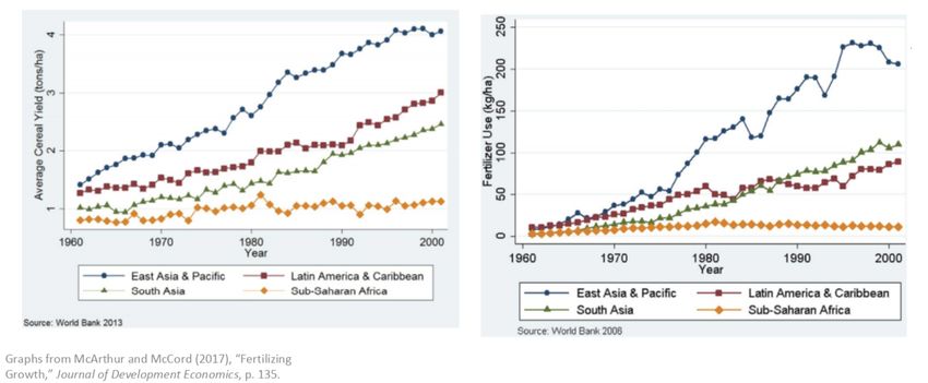
Bergquist (U Mich) STEG Macro Development April 1, 2021 27Speed of learning
Bergquist (U Mich) STEG Macro Development April 1, 2021 28Speed of learning
∼ 60% of the samples located in the range where learning is weak
Bergquist (U Mich) STEG Macro Development April 1, 2021 29Peer learning (Beaman et al., 2021)
But can’t people learn more quickly if learn from peers?
Bergquist (U Mich) STEG Macro Development April 1, 2021 30Peer learning (Beaman et al., 2021)
But can’t people learn more quickly if learn from peers?
And can targeting speed up peer learning?
Bergquist (U Mich) STEG Macro Development April 1, 2021 30Peer learning (Beaman et al., 2021)
But can’t people learn more quickly if learn from peers?
And can targeting speed up peer learning?
Simple contagion (λ = 1): an agent adopts as long as one of her
peers adopts
Complex contagion (λ ≥ 2): an agent adopts as long as λ of their
peers adopt
Now consider an intervention that aims to reach 2 “seed farmers” in
each network. The optimal entry points will depend on the contagion
model
Simple: first seed in dense part of network, second seed to diffuse to
the more distant periphery
Complex (λ = 2): choose both seeds in central part of the network
Bergquist (U Mich) STEG Macro Development April 1, 2021 30Adoption of pit-planting in Malawi
Nice features of the papers
Collect complete network data in 200 villages (Chandrashekar and
Lewis, 2011)
Simulate the various models to identify optimal entry points and then
experimental treatment are based on the models
Treatments vary at the village level based on the model used to select
seed farmers
Simple contagion
Complex contagion based on network data
Complex contagion based on geographical proximity network
Selection made by extension officers (status quo)
Bergquist (U Mich) STEG Macro Development April 1, 2021 31Seed farmers under different scenarios
Village 87 Village 141
Village 288
Legend
Simple
Complex
Geo
Simple & Complex
None
Note: some overlap.
Bergquist (U Mich) STEG Macro Development April 1, 2021 32Adoption by non-seed farmers: individual-level regs
Table 5: Diffusion Within the Village
Heard of PP Knows how to PP Adopts PP
(1) (2) (3) (4) (5) (6) (7) (8) (9)
Connected to 1 seed 0.002 0.030 0.016 0.017 0.021 -0.031 0.008 0.012 0.004
(0.024) (0.022) (0.029) (0.016) (0.017) (0.023) (0.011) (0.015) (0.017)
Connected to 2 seeds 0.084 ** 0.124 *** 0.064 0.062 ** 0.068 ** 0.110 ** 0.016 0.039 ** 0.014
(0.038) (0.040) (0.064) (0.028) (0.029) (0.051) (0.014) (0.019) (0.035)
Within path length 2 of at least -0.018 0.016 0.067 0.005 0.022 0.028 0.013 0.022 * 0.037 *
one seed (0.028) (0.027) (0.042) (0.018) (0.021) (0.028) (0.008) (0.013) (0.021)
Season 1 2 3 1 2 3 1 2 3
N 4155 4532 3103 4155 4532 3103 4203 3931 2998
Mean of Reference Group
0.223 0.286 0.391 0.057 0.095 0.147 0.013 0.044 0.043
(No connection to any seed)
SD of Reference Group 0.416 0.452 0.488 0.232 0.293 0.355 0.113 0.206 0.203
p-value for 2 connections = 1
0.018 0.013 0.442 0.072 0.091 0.004 0.522 0.164 0.760
connection
Notes
1 Sample excludes seed and shadow farmers. Only connections to simple, complex and geo seed farmers are considered (no connections to benchmark farmers
included).
2 The dependent variable in columns (1)-(3) is an indicator for whether the respondent reported being aware of a plot preparation method other than ridging and
then subsequently indicated awareness of pit planting in particular. In columns (4)-(6), the dependent variable is an indicator for whether the farmer reported
knowing how to implement pit planting. The dependent variable in (7)-(9) is an indicator for the household having adopted pit planting in that season.
3 In all columns, additional controls include indicators for the respondent being connected to: one Simple partner, two Simple partners, one Complex partner, two
Complex partners, one Geo partner, two Geo partners, within 2 path length of a Simple partner, within 2 path length of a Complex Partner, and within 2 path
length of the geo partner.
4 Also included in both panels are village fixed effects. Standard errors clustered at the village level.
5 The reference group is comprised of individuals with no direct or 2-path-length connections to a seed farmer.
6 *** pAdoption by non-seed farmers: village-level regs
Table 6: Village-Level Regressions of Adoption Outcomes Across Treatment Arms
Any Non-Seed Adopters Adoption Rate
(1) (2) (3) (4)
Simple Contagion Treatment 0.155 0.189 * 0.036 ** 0.006
(0.100) (0.111) (0.017) (0.022)
Complex Contagion Treatment 0.252 *** 0.304 *** 0.036 ** 0.036
(0.093) (0.101) (0.016) (0.026)
Geographic treatment 0.107 0.188 * 0.038 0.013
(0.096) (0.110) (0.027) (0.034)
Year 2 3 2 3
N 200 141 200 141
Mean of Benchmark Treatment
0.420 0.543 0.038 0.075
(omitted category)
SD of Benchmark 0.499 0.505 0.073 0.109
p-values for equality in coefficients:
Simple = Complex 0.300 0.240 0.981 0.173
Complex = Geo 0.102 0.220 0.937 0.491
Simple = Geo 0.623 0.990 0.950 0.783
Notes
1 The reference group is the Benchmark treatment.
2 The adoption rate in columns (1)-(2) include all radomly sampled farmers, excluding seed and shadow
farmers. The "Any non-seed adopters" indicator in columns (3)-(4) excludes only seed farmers.
3 Sample for year 3 (columns 2 and 4) excludes Nkhotakota district.
4 All columns include controls used in the re-randomization routine (percent of village using compost at
baseline; percent village using fertilizer at baseline; percent of village using pit planting at baseline);
village size and its square; and district fixed effects. Standard errors are clustered at the village level.
5 *** pFor more on info constraints
Learning can be helped or hampered depending on the gender of the
communicator (BenYishay et al. 2016, Kondylis et al. 2016)
With financial incentives, farmers selected by peers can encourage
greater adoption than a lead farmer selected by extension agents, but
without these incentives, the lead farmer outperforms the peer
farmers (BenYishay & Mobarak, 2017)
Farmers are more likely to adopt new seeds when when their land
quality is more similar to their peers who (randomly) receive new
seeds (Tjernstrom, 2017)
Mobile phone-based farming advice lines can increase farmers use of
fertilizer and encourage crop diversification (Cole & Fernando, 2012)
Bergquist (U Mich) STEG Macro Development April 1, 2021 35Outline
A model of agricultural technology adoption (Magruder 2018)
Where we have good micro evidence (for macro to build on):
Credit and risk inefficiencies (Karlan et al., 2014)
Informational inefficiencies (Bold et al, 2017; Beaman et al., 2021)
Where we have less micro evidence (and where macro can help):
Externalities/GE effects (Burke et al., 2019)
Comment on potential synergies between micro and macro
Bergquist (U Mich) STEG Macro Development April 1, 2021 36Large, Regular Seasonal Price Fluctuations
Study site
130 Eldoret
125 Kampala
125
120 Uganda 120
Kenya
Price index
Price index
115 115
110 110
Main maize 105
105 harvest
100
100
Jan Apr Jul Oct
Jan Apr Jul Oct Rwanda
125
Kisumu
Kigali 120
Price index
115
115
Tanzania
110 110
Price index
105
105
100
100 Jan Apr Jul Oct
Jan Apr Jul Oct
150 Mbeya
120 120 Arusha
US corn 140
115 115
Price index
130
Price index
Price index
110 120 110
105 110 105
100 100 100
Jan Apr Jul Oct Jan Apr Jul Oct Jan Apr Jul Oct
Bergquist (U Mich) STEG Macro Development April 1, 2021 37Storage
So: staple food prices not fixed within the season.
Storage should allow the movement of grain intertemporally
An unconstrained intertemporal profit maximizer should store a unit of
grain if:
δE [pt+1 ] > pt + c (1)
You might think: use storage to buy low, sell high
Bergquist (U Mich) STEG Macro Development April 1, 2021 38Instead: Sell Low, Buy High
Sell low, buy high: farm households appear to be selling low at harvest or
buying high later in the season – and often both
Inventories Quantity sold minus purchased
8
4
6
2
bags/week
bags
4
0-2
2
-4
0
0 10 20 30 0 10 20 30
weeks post harvest weeks past harvest
⇒ Modal HH in our sample appears to be giving up equivalent of 1-2
months of agricultural wages by selling low/ buying high, instead of the
reverse
Bergquist (U Mich) STEG Macro Development April 1, 2021 39Paper Overview
Why are farmers not using storage to arbitrage these price fluctuations?
Bergquist (U Mich) STEG Macro Development April 1, 2021 40Paper Overview
Why are farmers not using storage to arbitrage these price fluctuations?
Most common answer from farmers: credit constraints Other Explanations
Bergquist (U Mich) STEG Macro Development April 1, 2021 40Paper Overview
Why are farmers not using storage to arbitrage these price fluctuations?
Most common answer from farmers: credit constraints Other Explanations
High harvest-time expenditure needs must be funded by harvest-time
sales
Bergquist (U Mich) STEG Macro Development April 1, 2021 40Paper Overview
Why are farmers not using storage to arbitrage these price fluctuations?
Most common answer from farmers: credit constraints Other Explanations
High harvest-time expenditure needs must be funded by harvest-time
sales
We randomly offer a harvest-time loan to smallholder farmers (∼ $100)
Loan offer is randomized across farmers
Density of treatment is randomized across locations
Data:
Three rounds of household surveys throughout the year
Monthly price data at 52 local markets
Study timeline:
Two years of replication
Long-run follow-up survey 1-2 years after loan ended
Bergquist (U Mich) STEG Macro Development April 1, 2021 40Experimental Design
High intensity Low intensity
Sublocation-level
randomization
High intensity = 9 locations
Low intensity = 8 locations
Bergquist (U Mich) STEG Macro Development April 1, 2021 41Experimental Design
High intensity Low intensity
Sublocation-level
randomization
High intensity = 9 locations
Low intensity = 8 locations
c
Bergquist (U Mich) STEG Macro Development April 1, 2021 42Experimental Design
High intensity Low intensity
Sublocation-level
randomization
High intensity = 9 locations
Low intensity = 8 locations
c
Group-level
randomization Treatment Control Treatment Control
Y1 Y2 Timeline Balance
Bergquist (U Mich) STEG Macro Development April 1, 2021 43Individual Level Effects: Graphical Results
Inventories Net Revenues
4000
3
Pt Est 95% CI 90% CI Pt Est 95% CI 90% CI
2
Net Revenues, T - C
2000
Inventories, T - C
0 1
0
-1
-2000
-2
Nov Dec Jan Feb Mar Apr May Jun Jul Aug Sep Nov Dec Jan Feb Mar Apr May Jun Jul Aug Sep
Total HH consumption (log)
.4
Pt Est 95% CI 90% CI
Total HH consumption (log), T - C
0 .2
-.2
Nov Dec Jan Feb Mar Apr May Jun Jul Aug Sep
Bergquist (U Mich) STEG Macro Development April 1, 2021 44Individual Level Effects: Regression Results
Inventory Net Revenues Consumption
Overall By rd Overall By rd Overall By rd
Treat 0.56∗∗∗ 533.44∗∗∗ 0.04
(0.10) (195.49) (0.02)
Treat - R1 1.05∗∗∗ -613.58∗∗ 0.01
(0.18) (271.61) (0.03)
Treat - R2 0.55∗∗∗ 1187.97∗∗∗ 0.05∗
(0.12) (337.41) (0.03)
Treat - R3 0.09 998.67∗∗∗ 0.04
(0.16) (291.06) (0.03)
Observations 6780 6780 6730 6730 6736 6736
Mean DV 2.16 2.16 -1616.12 -1616.12 9.55 9.55
SD DV 3.23 3.23 6359.06 6359.06 0.64 0.64
R squared 0.33 0.33 0.12 0.12 0.06 0.06
Specification Other Results
Bergquist (U Mich) STEG Macro Development April 1, 2021 45Market Effects: Predictions
By encouraging greater storage, the loan shifted supply at different points
in the season. Does this affect local market prices?
Bergquist (U Mich) STEG Macro Development April 1, 2021 46Market Effects: Predictions
By encouraging greater storage, the loan shifted supply at different points
in the season. Does this affect local market prices?
When more individuals engage in arbitrage, we predict that:
Bergquist (U Mich) STEG Macro Development April 1, 2021 46Market Effects: Predictions
By encouraging greater storage, the loan shifted supply at different points
in the season. Does this affect local market prices?
When more individuals engage in arbitrage, we predict that:
Prices will be higher immediately after harvest, as maize in storage
rather than on market
Prices will be lower later, as stored maize is released
Bergquist (U Mich) STEG Macro Development April 1, 2021 46Market Effects: Graphical Results
Bergquist (U Mich) STEG Macro Development April 1, 2021 47Implications for Individual Returns to Storage
What do these GE effects mean for the individual returns to the loan?
Bergquist (U Mich) STEG Macro Development April 1, 2021 48Implications for Individual Returns to Storage
What do these GE effects mean for the individual returns to the loan?
The loan is designed to enable farmers to arbitrage seasonal price
variation
Bergquist (U Mich) STEG Macro Development April 1, 2021 48Implications for Individual Returns to Storage
What do these GE effects mean for the individual returns to the loan?
The loan is designed to enable farmers to arbitrage seasonal price
variation
High density areas see (significantly) higher post-harvest prices and
(weakly) lower lean-season prices
These price effects might diminish the profitability of storage, reducing
the benefit to the treated
N.B. smoother prices could benefit non-borrowers!
To explore this, estimate:
Yijry = α + β1 Tjy + β2 His + β3 Tjy ∗ His + ηry + εijry
Bergquist (U Mich) STEG Macro Development April 1, 2021 48Treatment Spillovers
(1) (2) (3)
Inventory Net Revenues Consumption
Treat 0.74∗∗∗ 1101.39∗∗ -0.01
(0.15) (430.09) (0.02)
Hi 0.02 164.94 -0.05
(0.24) (479.68) (0.04)
Treat * Hi -0.29 -816.77 0.07∗
(0.19) (520.04) (0.04)
Observations 6780 6730 6736
Mean DV 2.59 -1055.15 9.54
R squared 0.29 0.09 0.03
p-val T+TH=0 0.01 0.41 0.08
Effects by year IV Effects
Bergquist (U Mich) STEG Macro Development April 1, 2021 49Implications
Revenue effects are concentrated among low-intensity treated
individuals
Arbitrage is most profitable when you are the only one doing it
Bergquist (U Mich) STEG Macro Development April 1, 2021 50Implications
Revenue effects are concentrated among low-intensity treated
individuals
Arbitrage is most profitable when you are the only one doing it
Methodologically, impacts captured in a small pilots may not
correspond to impacts at scale
We would have overestimated the direct impacts of credit if evaluated
just among a few farmers
What implications do GE effects have for the distribution of gains?
Small indirect gains per-person could be a large part of the total gains
In this context, high saturation appears to provide larger social gains
but lower private gains
Gains Distribution
Bergquist (U Mich) STEG Macro Development April 1, 2021 50Outline
A model of agricultural technology adoption (Magruder 2018)
Where we have good micro evidence (for macro to build on):
Credit and risk inefficiencies (Karlan et al., 2014)
Informational inefficiencies (Bold et al, 2017; Beaman et al., 2021)
Where we have less micro evidence (and where macro can help):
Externalities/GE effects (Burke et al., 2019)
Comment on potential synergies between micro and macro
Bergquist (U Mich) STEG Macro Development April 1, 2021 51“From Micro to Macro Development”
Buera, Kaboski, and Townsend (2021):
Each has their strengths:
Micro: causality revolution (e.g. RCTs), deeply grounded in realities
and data of developing countries
Macro: focused on policies that have aggregate or economy-wide
distributional and welfare implications
Common (though not inherent) critiques:
Micro: not enough focus on aggregate effects at scale, disconnect from
theory
Macro: rely on strong structural assumptions, calibrated parameters
may not be well-identified or locally relevant
Bergquist (U Mich) STEG Macro Development April 1, 2021 52“From Micro to Macro Development”
Buera, Kaboski, and Townsend (2021):
Each has their strengths:
Micro: causality revolution (e.g. RCTs), deeply grounded in realities
and data of developing countries
Macro: focused on policies that have aggregate or economy-wide
distributional and welfare implications
Common (though not inherent) critiques:
Micro: not enough focus on aggregate effects at scale, disconnect from
theory
Macro: rely on strong structural assumptions, calibrated parameters
may not be well-identified or locally relevant
Methodological tools to bridge the gap:
Randomized saturation
Randomization at scale
Embedding RCTs/natural experiments in structural models
Bergquist (U Mich) STEG Macro Development April 1, 2021 52Examples from agricultural tech adoption
Burke at el (2019): storage loans shift supply of grain across time,
dampening seasonal price fluctuations
Fink et al (2020): seasonal loan to farmers increase on-farm labor and
agricultural output, driving up wages in local labor markets
Brooks and Donovan (2020): bridges lower risk of market access,
affects labor market choices, farm investment, and savings
Caunedo and Kala (2020): farm mechanization reduces labor
demand, including family labor in supervision activities
Casaburi and Willis (2020): randomizing subsidies to rent out land
Bergquist et al (2020): agriculture policies at scale can shift wages
and output prices, changing their average and distribution impacts
Your paper next...
Bergquist (U Mich) STEG Macro Development April 1, 2021 53Substantial variation in input quality
(N.B. Other studies find limited evidence of adulteration, e.g. Michelson et al. (2021))
Back
Bergquist (U Mich) STEG Macro Development April 1, 2021 54But not much variation in price
Back
Bergquist (U Mich) STEG Macro Development April 1, 2021 55Quality matters for yields
Do consumers not care about quality?
Bold et al. run agronomic trials to experimentally vary inputs
40% loss in yields at average input quality (retail hybrid, 32%N vs.
authentic hybrid, 46%N)
Back
Bergquist (U Mich) STEG Macro Development April 1, 2021 56Returns to retail and authentic input use
Back
Bergquist (U Mich) STEG Macro Development April 1, 2021 57Inference problem
Back
Bergquist (U Mich) STEG Macro Development April 1, 2021 58A model of learning about quality
Consider a farmer who wants to adopt fertilizer and starts
experimenting with it on a small plot.
The farmer knows that fertilizer of sufficiently high quality, say, with a
rate of dilution θ < θ∗ , where θ∗ is the threshold level, is profitable.
However, the dilution level θ ∈ 0, 1 is unknown
The farmer must therefore infer quality based on the yields on her
plot using Bayes’ rule
Bergquist (U Mich) STEG Macro Development April 1, 2021 59Characteristics of Seed Farmers
Table 1: Characteristics of the Seeds Chosen by Each Treatment Arm
Wealth Measures Social Network Measures
Farm Total Index Betweenness Eigenvector
Degree
Size (PCA) Centrality Centrality
(1) (2) (3) (4) (5)
Treatment arm:
Simple Contagion -0.152 0.113 0.455 156.009 ** 0.009
(0.19) (0.23) (1.03) (67.93) (0.01)
Complex Contagion -0.037 0.380 3.725 *** 146.733 ** 0.064 ***
(0.19) (0.23) (1.02) (67.74) (0.01)
Geographic -0.614 *** -0.740 *** -3.616 *** -90.204 -0.046 ***
(0.19) (0.23) (1.03) (68.04) (0.01)
p-values for tests of equality in seed characteristics
Simple = Complex 0.335 0.067 0.000 0.815 0.000
Complex = Geographic 0.000 0.000 0.000 0.000 0.000
Simple = Complex = Geographic 0.000 0.000 0.000 0.000 0.000
N 1248 1248 1232 1232 1232
Mean Value for Seeds in Benchmark Treatment
(omitted category) 2.06 0.626 11.9 169 0.173
SD for Seeds in Benchmark Treatment 2.97 1.7 6.77 343 0.0961
Notes
1 The sample includes all seeds and shadows. The sample frame includes 100 Benchmark farmers (2 partners in 50 villages), as we only observe
Benchmark farmers in Benchmark treatment villages, and up to 6 additional partner farmers (2 Simple partners, 2 Complex partners, and 2
Geo partners) in all 200 villages.
2 Benchmark treatment seeds are the omitted category.
3 *** pAdoption Rates for Seed Farmers (Relative to Shadow)
Table 2: Adoption Rates of Actual Seeds Relative to Shadow (Counterfactual) Farmers
Adopted Crop Residue
Adopted Pit Planting
Management
(1) (2) (3) (4) (5)
Seed 0.258 *** 0.230 *** 0.183 *** 0.137 *** 0.047
(0.03) (0.03) (0.04) (0.04) (0.04)
N 686 672 490 686 467
Mean of Shadows 0.054 0.093 0.139 0.320 0.207
Season 1 2 3 1 2
Notes
1 Also included are village fixed effects. Sample includes only seed farmers (chosen by the simulations and
trained on the technologies through our intervention) and shadow (counterfactual) farmers with the same
network characteristics but not trained by the experiment. The sample excludes Benchmark villages. Standard
errors are clustered at the village level.
2 *** pAdoption by Seed Farmersby Treatment Group
Table 3: Difference in Adoption Rates Across Seed Farmers chosen through Different Targeting Strategies
Adopted Crop Residue
Adopted Pit Planting
Management
Treatment: (1) (2) (3) (4) (5)
Simple Contagion -0.006 0.129 * 0.176 ** 0.078 -0.097
(0.07) (0.07) (0.09) (0.08) (0.09)
Complex Contagion -0.020 0.002 0.037 -0.001 -0.077
(0.08) (0.07) (0.08) (0.08) (0.09)
Geographic -0.095 -0.064 -0.003 -0.011 -0.075
(0.08) (0.07) (0.08) (0.08) (0.10)
N 353 352 259 353 243
Mean Adoption for Seeds in Benchmark
0.337 0.276 0.238 0.442 0.339
Treatment (the omitted category)
p-value for tests of equality in adoption rates across treatment cells:
Simple = Complex 0.862 0.077 0.108 0.311 0.808
Complex = Geographic 0.360 0.358 0.625 0.886 0.977
Joint test of 3 treatments 0.252 0.008 0.049 0.235 0.795
Season 1 2 3 1 2
Notes
1 Also included are stratification controls (percent of village using compost at baseline; percent village using fertilizer at baseline; percent
of village using pit planting at baseline); village size and its square; and district fixed effects. Only seed farmers chosen by our
interventions to be trained on the technologies are included. Standard errors are clustered at the village level.
How does this affect our interpretation of the results?
2 *** pYou can also read