Empirical forward price distribution from Bitcoin option prices
←
→
Page content transcription
If your browser does not render page correctly, please read the page content below
Empirical forward price distribution from Bitcoin option prices
                                                                                          Nikolai Zaitsev∗

                                                                                           12 Jan 2019
arXiv:1901.04770v1 [q-fin.ST] 15 Jan 2019

                                                                                             Abstract
                                                          Report presents analysis of empirical distribution of future returns of bitcoin (BTC)
                                                      from BTUSD inverse option prices. Logistic pdf is chosen as underlying distribution
                                                      to fit option prices. The result is satisfactory and suggests that these prices can be
                                                      described with just three or even one parameter. Fitted Logistic pdf matches forward price
                                                      movements upto a scaling factor. Nevertheless, this observation stands alone and does
                                                      not allow stochastic description of underlying prices with logistic pdf in similar fashion
                                                      as it is done within Black-Scholes modelling framework. Put-call parity relationship is
                                                      derived connecting prices of vanilla inverse options and futures.

                                            1        Introduction
                                            1.1        Crypto market and Bitcoin (BTC) options
                                            Crypto coins market is quite new, however, due to the recently inflated bubble peaked to the
                                            size of $800 billion and then imploded to the level of $100 billion it attracted great attention
                                            from investors. Barely noticed 4-5 years ago it is considered today as an asset class attractive
                                            for investments. Despite such attention, it still lacks official recognition by the governmental
                                            authorities.
                                                Bitcoin (BTC) is the first and the most popular crypto coin. It consistently leads all other
                                            coins by the market capitalization and trading volume. It is traded against fiat currencies,
                                            such as dollar (USD), euro (EUR), sterling pound (GBP) and many others across multiple
                                            exchanges (for example, see the list at [1] or [2]. BTC is attractive due to various reasons,
                                            where a possibility for direct transactions between two counterparts (P2P transactions) and
                                            strictly controlled inflation of monetary base are the major one. Since Bitcoin regulation and
                                            legal protection are still in their infancy it is vulnerable to price manipulation either from
                                            media or from traders with large financial resources. As result, BTC exchange rate is volatile
                                            with sharp jump-like movements. Such dynamics creates demand from crypto investors for
                                            hedging their risks and for pure speculations.
                                                ∗
                                                    Director of UXTA.io and INNOVAEST.ORG. Correspondent e-mail: nikzaitsev@yahoo.co.uk

                                                                                                  1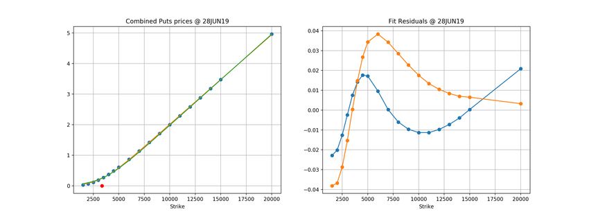
This demand stimulates foundation of derivative exchanges supporting public trading
in options, futures, perpetuals, CFD’s, swaps and other products. For example, BTCUSD
Futures are traded also at CBOE (Chicago Board Option Exchange) within regulated envi-
ronment. This report focuses on options. So far only three option exchanges are known:
        • Deribit ( https://deribit.com )

        • Quedex ( https://quedex.net )

        • LedgerX ( https://ledgerx.com )
     They all support trading of options and futures, however they differ in data policy. Deribit
exchange has open data policy and allows very simple download of snapshot of option and
futures prices in the trading book. Information of trading book of Quedex requires registration
and some additional programming effort, however, it is also open. LedgerX is an OTC
platform targeting large investors. Their data is not publicly available. This report uses
Deribit data only.
     Aim of this report is extraction of forward-looking price distribution from analysis of
option prices. Its purpose is to give reader an impression about market sentiments and
provide tools for evaluation of risks present in the market. To give more faith to this analysis
the report gives a brief description about what options do.
     This report is based on the analysis of empirically observed market data and tries to follow
model free path. The results are fit to logistic distribution function, which is not commonly
used in financial mathematics. The resulting fit is surprisingly good. Solution of this puzzle
is left beyond this article, which aims only to report the observed fact.

2        Contract definitions
Option is a contract allowing buyer the right to receive payments according to the predefined
payout formula. This formula is calculated at the settlement which occurs at Maturity date.
Price of Underlying at Maturity is input to the formula applied. This report discusses vanilla
European Put and Call options and BTCUSD as Underlying. Deribit exchange is marketing
contracts settled at specified maturities in accord to its Type (Call or Put) and Strike. Before
maturity, the contracts may change hands via trading between clients of exchange. Number
of contracts circulating around is named Open interest and is specified per type and strike.
Open interest is not included into analysis presented in this report.
    Strike level is expressed in USD paid for 1 BTC (i.e. BTCUSD exchange rate). Option
price is settled ”physically” i.e. the account is always debited or credited in units of BTC.
This happens since many crypto exchanges operate outside of any regulations.
    BTC is not exchanged for USD at Deribit. Instead the exchange uses external quote.
Since BTC price is subject to large jumps, Deribit uses an average of rates quoted at few
liquid exchanges, such as Bitstamp, GDAX (Coinbase), Gemini, Itbit, Kraken and Bitfinex 1 .
    1
        during observation period presented in this paper, Deribit did not include Bitfinex into the average

                                                          2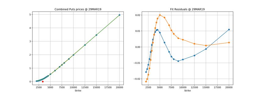
The averaging algorithm is explaned as follows:

    • 6 online: we leave the highest and lowest and each exchange accounts for 25%

    • 5 online: we leave the highest and lowest and each exchange accounts for 33.33%

    • 4 online: we leave the highest and lowest and each exchange accounts for 50%

    • 3 online: each exchange accounts for 33.33%

    • 2 online: each exchange accounts for 50%

    • 1 online: exchange represents the index

3    Mathematical definitions
At Deribit call (put) is defined as a contract where buyer has a right to buy (sell) the un-
derlying, x, at fixed price level called strike, K. At the time of maturity (t = T ) buyer
may execute this right only if price of underlying, xT , is above (below) strike level for call
(put). Options deliver bitcoins (BTC) while underlying and strike are expressed in terms of
underlying exchange rate. The payout of call is defined as:

                                         max(0, xT − K)   (xT − K)+
                          C(xT , K) =                   =                                      (1)
                                              xT              xT
Similarly, payout of put is defined as:

                                         max(0, K − xT )   (K − xT )+
                          P (xT , K) =                   =                                     (2)
                                              xT              xT

   On the other side of the contract, call (put) seller (also underwriter) is obliged to sell (buy)
the Underlying at price defined by the Strike. Options and futures are settled in bitcoins.
Because of that we see two consequences:

    • non-zero part of option payout is non-linear.

    • No fiat currency, such as USD, is involved in the exchange of funds between traders.
      Hence, USD account is excluded from further consideration.

4    Properties of option prices
From the definition of payout one can derive one useful relationship named put-call parity.
Commonly used notations are:

    • At-the-money (ATM) level. It is the level where the future x price is equal to strike, K.

                                                3
• In-the-money (ITM) option is call (put) option where price of underlying is significantly
larger (less) than strike. In this case, there is very high correlation between movements
of option price and price of underlying.
• Out-the-money (OTM) option is a call (put) option where price of underlying is sig-
nificantly less (larger) than Strike. In this case, the correlation between movements of
option price and price of underlying is very low.
4.1 Put-call parity
It is easy to infer that under any circumstances at Maturity we will have the following:
(xT − K)+ (K − xT )+
C(xT , K, T ) − P (xT , K, T ) = −
xT xT
(3)
xT − K
C(xT , K, T ) − P (xT , K, T ) =
xT
This relationship is called put-call parity and it is also valid any moment before maturity.
This fact can be rewritten in terms of expectations. Since the future price outcome is not
known one can apply expectation operator Et [.] to both sides:
xT − K
Et [C(xT , K, T )] − Et [P (xT , K, T )] = Et [ ]
xT
(4)
1
= 1 − K · Et [ ]
xT
Eq. 3 and Eq. 4 become equivalent at t = T . Further we use that Et [C(x, K, T )] = C(x, K, t):
1
C(x, K, t) − P (x, K, t) = 1 − K · Et [ ] (5)
xT
BTC has no discount mechanism due to no embedded inflation. To calculate expectation of
inverted value we have to define inverse futures [3], non-linear products, traded at the same
exchange 2 :
1 1
= Et [ ] (6)
Ft xT
Finally, substitute, this expression into Eq. 5:
K
C(xt , K, t) − P (xt , K, t) = 1 − (7)
Ft
This relationship does not depend on evolution of underlying. Eq. 7 is one of results of this
note written for ’inverted’ options and futures on BTC. Note, the unusual for put-call parity
relationship between Long Call, Short Put and inverse futures. That is because of the physical
settlement feature of these contracts.
2 1 (y)
It is derived, by looking from bitcoin perspective, where yt = xt
. Without discount we have Ft =
(y)
Et [yT ] = yt . Hence, Ft = 1/Ft
44.2 Expected future distribution of BTC
Beliefs of people about different outcome of xT given current observation of xt is reflected
through option prices they are quoting and subsequently trade. To see that we have to define
a function of probability to observe price of underlying of xT at maturity given the initial
value of xt : f (xT |xt ). The expectation operator used above can be rewritten as (use call as
an example):
Z +∞
Et [C(xT , K, T )] = Ct (xt , K, t) = (1 − K/xT )+ · f (xT |xt ) · dxT
−∞
Z +∞ (8)
= (1 − K/xT ) · f (xT |xt ) · dxT
K
Function f (xT |xt ) follows properties of probability function and can be interpreted as
a probability to find a person who ’believes into’ xT given spot value xt . People within
marketplace negotiate between each other in accordance to their view of the future, where
the option price results in the recorded trade. Hence, option price as a function of strike, K,
and of spot price, xt , contains information about distribution of underlying which is believed
by traders to be at t = T . There is simple model independent approach to extract this
information. Note, that Eq. 8 is written without making any specific assumptions about
shape of f (x). By taking first derivative of call price function with respect to strike we find
that:
dCt (xt , K) 1
= · (1 − CDF (xT = K|xt )) (9)
dK xT
By taking second derivative one can observe the result from Breeden and Litzenberger [4],
which is distribution of future BTC price:
d2 Ct (xt , K) f (xT = Kxt )
= (10)
dK 2 xT
Similar expression is true for puts.
4.3 Logistic distribution
So far, there was no assumption about the shape of f (x). Log-Normal distribution is used
more frequently as it lays the basis under modern option pricing theory. Original derivation
of Black-Scholes formula uses arbitrage-free arguments. This model introduces volatility as a
parameter, which is widely used in the investments and trading environment. At some point,
[5], it was found that volatility implied from option prices exhibits dependency on strike and
is asymmetric. This feature is called ”volatility smile”. Such behavior indicates that the
terminal p.d.f. (or f (x)) does not follow assumed Log-Normal distribution. In attempt to
resolve this issue empirically, let us look onto CDF properties, where:
5lim CDF (u) = 0
x→−∞
(11)
lim CDF (u) = 1
x→+∞
One may notice that CDF-function resembles sigmoid function, which is:
1
CDF (x, m, s) = x−m (12)
1 + e− s
The respective p.d.f. is referred as Logistic distribution, which is:
x−m
e− s
P DF (x, m, s) = f (x, m, s) = x−m (13)
s · (1 + e− s )2
By recalling the relationship between Eq. 9 and Eq. 10 one may naturally think to use sigmoid
to model CDF -function. The advantage of using sigmoid as CDF is that all its ”siblings”
(i.e. CDF (x), P DF (x)) have close-form. An integral of sigmoid (IS(x, m, s)) has closed-form
as well:
x−m
IS(x, m, s) = log (1 + e s ) · s (14)
Here we may interpret parameter m as AT M -level and s as a volatility. Considering these
similarities, further we use IS(x) to model Put price, i.e. IS(x) → Pth (x), as a function of
strike. Additional parameter a is added:
x−m
Pth (x, m, s) = log (1 + e s )·s·a (15)
This parameter is responsible for normalization of CDF, because: CDF (+∞) = a. In our
analysis all three parameters are left free. Model with two fixed parameters is also checked.
Let us apply this guess to the data.
5 Analysis
5.1 Data
Data used in this analysis, are downloaded from Deribit and are collected during a day at
5-minutes intervals. It has open REST feed, which delivers snapshot of limit order book for
options and futures quoted over all marketed Maturities. As of today, Deribit quotes two
futures with maturities in Dec18, and Mar19, while there are two option maturities in Dec18,
one in Jan19, Mar19 and Jun19, i.e. five option maturities in total.
Data were collected from 10-Dec-2018 to 16-Dec-2018.
65.2 At-the-money level
ATM level is equal to forward value of underlying. As a number this can be measured in
three ways:
• calculate forward value directly through discounted cash flows method (fair valuation).
• use observed futures prices at the same maturity as of options under question. Deribit
quotes less futures maturities than that for options.
• by using call-put parity one can build synthetic futures prices as function of strike and
find the zero price via linear regression. By put-call parity, it is futures price.
The latter method is used to imply ATM level (Et [1/xT ]−1 ) for all option maturities. See
Fig. 1, Right plot for illustration. Further we use ATM-level and not futures for two reasons:
• it is found empirically, through option prices, therefore, it is consistent with chosen set
of option prices
• there are more option maturities than futures maturities
Figure 1: Left: Call (blue) and Put (orange) bid and ask prices as function of strike. Green
line shows synthetic put mid prices, Pc (x). Right: Price of synthetic forward as Long Call
Short Put price as a function of strike. Options of maturity at 29-Mar-19 are used. Snapshot
is taken at 2018-Dec-11 04h:10m
5.3 Filter option prices
Both, call and put, prices contain the same information about future price of underlying.
Therefore, call prices are converted to put prices by using call-put parity:
K
Pc (x) = C(x) − 1 + (16)
AT M
7Maturity IP D, % m s a Res(×1000) Spr(×1000) s(single)
28-Dec-18 0.00 3.52 0.31 1.00 1.12 5.69 0.45
25-Jan-19 0.13 3.38 0.51 0.95 2.04 5.88 0.69
29-Mar-19 0.87 3.22 0.68 0.95 3.98 6.43 0.90
28-Jun-19 2.50 2.95 0.81 0.92 4.72 10.36 1.19
Table 1: Implied PD, parameters, fit residual and average bid-ask spread are shown for
different maturities. For fit stability, underlying prices were divided by 1000. m-parameter is
1000 smaller as it should be. s(single) is fit result of 1 parameter model.
See calls and puts prices on Fig. 1, Left plot for an illustration of the method.
As result of data cleansing, we have 4 points per strike, which are averaged into ”combined
put prices”. Resulting option prices require certain filtering. Although in general we find
smooth data, at night (all crypto exchanges operate on 24x7 basis) or during extreme price
movements quotes are moving away or even disappear. Only option prices with both ask
(sell) and bid (buy) quotes are used.
5.4 Fitting put prices to integral sigmoid
In the next step, integrated sigmoid from Eq. 15 is fitted to the combined put prices by using
Least Squares method (see Fig. 2 and Fig. 3). Two functions were applied. First, is when
all three parameters, m, s, a, are free. Second, is when only s-parameter is free and others
are fixed as a = 1 and m = AT M . First method has smaller residuals, but the second one
fits almost within bid-ask. This indicates that we can reduce option description to just two
parameters, AT M and s, one of which is ’almost’ observable and can be replaced with futures
price.
Prices fit integrated sigmoid very well. Average residual between data and theoretical
points is of the order or better than the average bid-ask spread of option quotes. This means
that all option prices per each maturity can be parameterized with just three parameters, m,
s and a or even with only one parameter. For details see Table below.
Span of p.d.f. into range of negative strikes may be interpreted as a possibility for BTC
to ”default”. Although BTC cannot default, this term might illustrate the situation where
BTC price may become (near) zero. For example, implied probability of default (IP D) for
distributions shown in Fig. 2 and Fig. 3, are 0.87% and 2.50% respectively. Summary of
findings for this snapshot is given in the Table 1:
Black-Scholes implied log-normal volatilities replicate the well-known ’volatility smile’ [5].
As an example, see Fig. 4.
’Volatility smile’ is an artifact of Black-Scholes model and makes option pricing a very
complicated technology. In order to replicate market prices, we have to build a complex
theoretical structure, like interpolations of volatility surfaces or capture of correlated dynamics
between volatilities and returns on forward prices. Use of ”Logistic distribution” makes
8Figure 2: Top-Left: Fit (line) of integrated sigmoid to combined put prices (dots). Top-Right:
Fit Residuals with respect to mid-prices for 3-parameter (msa) fit (Blue) and s-parameter fit
(Orange). Bottom: Respective p.d.f of forward BTCUSD for 3-parameter (msa) fit (Blue)
and s-parameter fit (Orange). Red point shows ATM-level. Options of maturity at 29-Mar-19
are used. Snapshot is taken at 2018-Dec-11 04h:10m
modeling significantly simpler.
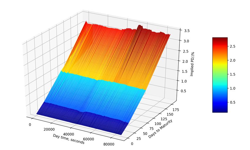
5.5 One day evolution of IPD
Analysis of dataset from 11-Dec-2018 allows to see stability of developed procedures and
certain correlations. Evolution of Implied PD’s as function of day time and days to maturity
is shown in Fig. 5
5.6 Correlations between parameters
Correlations between parameters are shown in Fig. 6 for completeness of results. s-parameter
moves together with m-parameter, where changes correlate at 68%, a-parameter is almost
9Figure 3: Top-Left: Fit (line) of integrated sigmoid to combined put prices (dots). Top-Right:
Fit Residuals with respect to mid-prices for 3-parameter (sma) fit (Blue) and s-parameter fit
(Orange). Bottom: Respective p.d.f of forward BTCUSD for 3-parameter (sma) fit (Blue)
and s-parameter fit (Orange). Red point shows ATM-level. Options of maturity at 28-Jun-19
are used. Snapshot is taken at 2018-Dec-11 04h:10m
constant as function of m-parameter. Ideally, we would want to fix m-parameter equal to
AT M and a-parameter equal to 1 (because of definition of probability) leaving s-parameter
as the only one free.
Single parameter model is not illustrated here.
5.7 Control of distributions
5.7.1 Comparison of model implied p.d.f. with future distribution
In order to validate interated sigmoid, IS(x), as function to fit option prices we can compare
implied p.d.f. with forward distribution of returns. For this purpose, for each moment in time
10Figure 4: Black-Scholes implied volatilities from options with maturities at 28-Jun-19 are
used. Snapshot data are taken at 2018-Dec-11 04h:10m
CDF (x) is implied from option prices and compared with forward return:
rF W D = AT Mt − AT Mt−1 (17)
, where AT Mt is implied from put-call parity and used as a proxy of futures. 5-minute returns
are used. Implied P DF is scaled down to 5-minute horizon from Maturity horizon by factor
p
equal to root square of time, (T − t)/5min. If return follows predicted distribution, then
we can write: r
T −t
P DF5m (x) ∼ P DF (x, m, s) · (18)
5min
Therefore,
−1
CDF5m (rF W D ) ∼ U (.) (19)
i.e. returns transformed with inverted implied CDF should follow uniform distributuon,
U(.).The result is shown below in Fig. 7. Data seem to not follow the prediction given by
options. By inroducing additional scaling factor to option implied distribution of η = 0.728 we
find that both forward returns and implied PDF follow similar shape, see Fig. 8. Kolmogorov-
−1
Smirnov p-value of comparison of CDF5m (rF W D ) to uniform distribution is 0.39. Scale η < 1
indicates that option impied PDF is wider than the real distribution of returns. It is a well
known fact for option traders who overprice their options with respect to historical (realised)
volatility to cover volatility of volatility risk.
11Figure 5: 283 snapshots at 5 minutes intervals from 11-Dec-2018 are analyzed. Implied PD
(vertical Z-axis) is presented as function of Daytime in seconds (X) and Number of days to
maturity (Y )
6 Logistic distribution as distribution of underlying process
6.1 New Parameters as risk factors
Parameters of presented logistic distribution, m, s, a, can be considered as new risk factors.
If so, they can be used in hedging risks and risk management framework. In this case, m can
be interpreted as forward price (or ATM) level. s can be used as replacement of volatility.
When m and a are fixed as described above in section 5.4 the model still provides satisfactory
results. Since sigmoid and its ’siblings’ are all expressed in closed form, the derivatives with
respect to these parameters can be used to manage option positions more accurately.
However, the above proposal should be used with care, because only consistent pricing
framework 3 can make these parameters the real new risk factors. Otherwise they can be
used only on the empirical basis.
6.2 Dynamics
Remember, that the pricing framework based on Black-Scholes model allows non-arbitrage
cross calibration of wide range of vanilla and exotic products with uniform interpretation of
implied volatilities. Since logistic distribution is not a stable distribution, the creation of
consistent pricing based on that seems to be very difficult at this point if not possible at all.
3
Black-Scholes framework is ’consistent’ in the sense that all products including exotics can be priced and
hence hedged with log-normal process of underlyiing which is shared among different products.
12Figure 6: Scatter plots of parameters. Left: s- vs m-parameters and Right: a- vs m-
parameters. Data for options with maturity in March from 11-Dec-2018 are used.
Also, under Central Limit Theorem the distribution of returns simulated as dr = µ · dt + dLD,
where dLD ∼ Logistic(x), will converge to the Normal distribution. This problem remains
unsolved. So far the the only way to make logistic distribution stable again is to combine it
with geometric distribution as it is proposed in [6]. We do not see how this operation can be
easily connected with trading mechanisms.
6.3 Other asset classes
The same logistic distribution was briefly applied to american equity options (e.g. Microsoft,
MSFT traded at NASDAQ). The resulting fit was good with similar quality. Interest rate
Swaptions (IR options on swaps as underlying) were also investigated with this method. The
result is also satisfactory upto maturities and terms of underlying swaps of less than 20 years.
From this we would like to cautiously conclude that this finding is universal. More analysis
has to be performed to confirm this statement.
7 Conclusion
Analysis of BTC option prices is presented. We propose new method to describe option prices
with integral sigmoid, which is CDS of logistic distribution. The analysis demonstrates great
stability and ability to interpret parameters of this model. This parameterisation employs only
3 parameters. Model with only one free parameter is also satisfactory. Option implied PDF
is compared to forward price movement and perfect agreement is found. It is still a question
to answer whether this parameterization is due to ’pure luck’ or it has some understandable
dynamics, which can be used as an alternative to Black-Scholes log-normal model. Put-call
parity for inverse options and futures traded within BTC exchanges is derived.
13Figure 7: Left: QQ-plot of quantiles of probabilities of historical returns extracted from CDF
Implied from options (Y-axis) vs Uniform quantiles. Right: Option prices with Maturity of
Jan-25-2019 are used. 1747 snapshots from 08-Dec-2018 to 18-Dec-2018 are analyzed
8 Acknowledgments
This work is self-funded and is done as a part of service advertised at UXTA.io. Although all
ideas and analysis presented in this paper are original, the author would like to thank Oleg
Nedbaylo for his support and collaboration in the development of algo-trading platform. This
idea came as a direct conqsequence of this partnership. Author also would like to express the
gratitude to Stefan Boor (Finmetrica Ltd) for proof reading and comments on the article. I
express many thanks to Cyril Shmidt (Abn-AMRO) who also challendged some derivations.
References
[1] list of bitcoin exchanges. at https://bitcoin.org/en/exchanges#international
[2] list of bitcoin exchanges. at https://coinmarketcap.com/exchanges/volume/
24-hour/
[3] ”Inverse Futures in Bitcoin Economy”, SSRN-2713755, 2015
[4] Breeden, D.; Litzenberger, R.. ”Prices of State-contingent Claims Implicit in Option
Prices”, Journal of Business, 51, pp. 621-651, 1978.
14Figure 8: Left: QQ-plot of quantiles of probabilities of historical returns extracted from CDF
Implied from options (Y-axis) vs Uniform quantiles. Right: Option prices with Maturity of
Jan-25-2019 are used. 1747 snapshots from 08-Dec-2018 to 18-Dec-2018 are analyzed.
[5] Derman, E.; I, Kani.. ”The Volatility Smile and Its Implied Tree”. RISK, issue 7-2, 1994,
pp. 139-145, pp. 32-39
15You can also read