Low frequency extrapolation with deep learning Hongyu Sun and Laurent Demanet, Massachusetts Institute of Technology
←
→
Page content transcription
If your browser does not render page correctly, please read the page content below
Low frequency extrapolation with deep learning
Hongyu Sun∗ and Laurent Demanet, Massachusetts Institute of Technology

SUMMARY                                                             ing in many fields, geophysicists have begun borrowing such
                                                                    ideas in seismic processing and interpretation (Chen et al.,
The lack of the low frequency information and good initial          2017; Guitton et al., 2017). Machine learning techniques at-
model can seriously affect the success of full waveform inver-      tempt to leverage the concept of statistical learning associated
sion (FWI) due to the inherent cycle skipping problem. Rea-         with different types of data characteristics. Lewis and Vigh
sonable and reliable low frequency extrapolation is in principle    (2017) investigate convolutional neural networks (CNNs) to
the most direct way to solve this problem. In this paper, we        incorporate the long wavelength features of the model in the
propose a deep-learning-based bandwidth extension method            regularization term, by learning the probability of salt geobod-
by considering low frequency extrapolation as a regression          ies being present at any location in a seismic image. Araya-
problem. The Deep Neural Networks (DNNs) are trained to             Polo et al. (2018) directly produce layered velocity models
automatically extrapolate the low frequencies without prepro-       from shot gathers with DNNs. Richardson (2018) constructs
cessing steps. The band-limited recordings are the inputs of the    FWI as recurrent neural networks.
DNNs and, in our numerical experiments, the pretrained neu-
ral networks can predict the continuous-valued seismograms          In the case of bandwidth extension, the data characteristics are
in the unobserved low frequency band. For the numerical ex-         the amplitudes and phases of seismic waves, which are dic-
periments considered here, it is possible to find the amplitude     tated by the physics of wave propagation. Among many kinds
and phase correlations among different frequency components         of machine learning algorithms, we have selected DNNs for
by training the DNNs with enough data samples, and extrapo-         low frequency extrapolation due to the increasing community
late the low frequencies from the band-limited seismic records      agreement (Grzeszczuk et al., 1998; De et al., 2011; Araya-
trace by trace. The synthetic example shows that our approach       Polo et al., 2017) in favor of this method as a reasonable surro-
is not subject to the structural limitations of other methods to    gate for physics-based process. The universal approximation
bandwidth extension, and seems to offer a tantalizing solution      theorem also shows that the neural networks can be used to
to the problem of properly initializing FWI.                        replicate any function up to our desired accuracy if the DNNs
                                                                    have enough hidden layers and nodes (Hornik et al., 1989).
                                                                    Although training is therefore expected to succeed arbitrarily
                                                                    well, only empirical evidence currently exists for the perfor-
INTRODUCTION                                                        mance of testing a network out of sample.

It is recognized that the low frequency data are essential for      In this paper, we choose to focus on CNNs. The idea behind
FWI since the low wavenumber components are needed for              CNNs is to mine the hidden correlations among different fre-
FWI to avoid convergence to a local minimum, in case the            quency components. The raw band-limited signals in the time
initial models miss the reasonable representation of the com-       domain are directly fed into the CNNs for regression and band-
plex structure. However, because of the acquisition limita-         width extension. The limitations of neural networks for such
tion and low-cut filters in seismic processing, the input data      signal processing tasks, however, are (1) the lack of general-
for seismic inversion are typically limited to a band above         izability guarantees and (2) the absence of a physical inter-
3Hz. With assumptions and approximations to make infer-             pretation for the operations performed by the networks. Even
ence from tractable but simplified models, geophysicists have       so, the preliminary results shown here for the synthetic dataset
started estimating the low wavenumber components from the           demonstrate a new direct method that attempts to extrapolate
band-limited records by signal processing methods. For exam-        the true values of the low frequencies rather than simply esti-
ple, they recover the low frequencies by the envelope of the        mating and compensating the low frequency energy.
signal (Wu et al., 2014; Hu et al., 2017) or the inversion of the
reflectivity series and convolution with the broadband source
wavelet (Wang and Herrmann, 2016; Zhang et al., 2017). How-         THEORY AND METHOD
ever, the low frequencies recovered by these methods are still
far away from the true low frequency data and can only be           A neural network defines a mapping y = f (x, w) and learns the
used during the construction of the initial model for FWI. Li       value of the parameters w that result in a good fit between x
and Demanet (2016) attempt to extrapolate the true low fre-         and y. DNNs are typically represented by composing together
quency data based on phase tracking method (Li and Demanet,         many different functions to find complex nonlinear relation-
2015). Unlike the explicit parameterization of phases and am-       ships. The chain structures are the most common structures in
plitudes of atomic events, here we propose an approach that         DNNs (Goodfellow et al., 2016):
deals with the raw band-limited records. The deep convolu-
                                                                                      y = f (x) = fL (... f2 ( f1 (x))),           (1)
tional neural networks (CNNs) are trained to automatically re-
cover the missing low frequencies from the input band-limited       where f1 , f2 and fL are the first, the second and the Lth layer of
data.                                                               the network. The overall length of the chain L gives the depth
                                                                    of the deep learning model. The final layer is the output layer,
Because of the state-of-the-art performance of machine learn-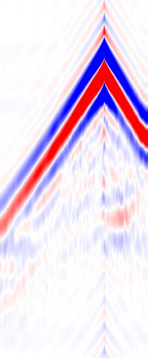
Low frequency extrapolation with deep learning

which defines the size and type of the output data. The training    One typical architecture of DNNs that uses the convolution to
sets specify directly what the output layer must do at each point   extract spatial features is CNNs. CNNs characterized by local
x but not specify the behavior of other layers. They are hidden     connections and weight sharing can exploit the local correla-
layers and computed by activation functions. The nonlinear-         tion of the input image. The hidden units are connected to a lo-
ity of the activation function enables the neural network to be     cally limited subset of units in the input, which is the receptive
a universal function approximator. Rectified activation units       field of the filter. The size of the receptive field increases as we
are essential for the recent success of DNNs because they can       stack multiple convolutional layers, so the CNNs can also learn
accelerate convergence of the training procedure. Numerical         the global features. The CNNs are normally designed to deal
experiment shows that, for bandwidth extension, Parametric          with image classification problems. For bandwidth extension,
Rectified Linear Unit (PReLU)(He et al., 2015) works better         the data to be learned are the one-dimensional time-domain
than the Rectified Linear Unit (ReLU). The formula of PReLU         seismic signals, so we directly consider the amplitude at each
is                                                                 sampling point as the pixel value of the image to be fed into
                              αy, i f y < 0                         the CNNs. The basic construction of CNNs in this paper is the
                g(α, y) =                        ,            (2)
                              y,     if y ≥ 0                       convolutional layer with N filters of size n × 1 followed by a
where α is also a learnable parameter and would be adaptively       batch normalization layer and a PReLU layer. The filter num-
updated for each rectifier during training.                         ber in each convolutional layer determines the number of the
                                                                    feature map or the channel of its output. Each output channel
Unlike the classification problem that trains the DNNs to pro-      of the convolutional layer is obtained by convolving the chan-
duce a probability distribution, regression problem trains the      nel of the previous layer with one filter, summing, adding a
DNNs for the continuous-valued output. It evaluates the per-        bias term. The batch normalization layer can speed up training
formance of the model by calculating the mean-squared error         of CNNs and reduce the sensitivity to network initialization
(MSE) of the predicted outputs f (xi ; w) and the actual outputs    by normalizing each input channel across a mini-batch. Al-
yi :                                                                though the pooling layer is typically used in the conventional
                             m
                          1X                                        architecture of CNNs, we leave it out because both the input
                J(w) =          L(yi , f (xi ; w)),          (3)
                         m                                          and output signals have the same length, so downsampling is
                                i=1
                                                                    unhelpful for bandwidth extension in our experiments.
where the loss L is the squared error between the true low
frequencies and the estimated outputs of the neural networks.       Since CNNs belong to supervised learning methods, we need
The cost function J is usually minimized over w by stochastic       to firstly train the CNNs from a large number of samples to de-
gradient descent (SGD) algorithm using a subset of the train-       termine the coefficients of the network, and, secondly, use the
ing set. This subset is called a mini-batch. Each evaluation        network for testing. According to the statistical learning the-
of the gradient using the mini-batch is an iteration. The full      ory, the generalization error is the difference between the ex-
pass of the training algorithm over the entire training set us-     pected and empirical error. It can be approximately measured
ing mini-batches is an epoch. The learning rate η (step-size)       by the difference between the errors on the training and test
is a key parameter for deep learning and required to be fine-       sets. For the purpose of generalization, the models to create the
tune. Adaptive moment estimation (Kingma and Ba, 2014) is           large training sets should be able to represent many subsurface
one of the state-of-the-art SGD algorithms which can adapt the      structures, including different types of reflectors and diffrac-
learning rate for each parameter by dividing the learning rate      tors, so we can find a common set of parameters for data from
for a weight by a moving average for that weight. Both of the       a specific region. The performance of the neural networks is
gradients and the second moments of the gradients are used to       sensitive to the architecture and hyperparameters, so we should
calculate the moving average.                                       design them carefully. Next, we illustrate the specific choice of
                                                                    the architecture and hyperparameters for bandwidth extension
                             m̂w
             wt+1 = wt − η √        ,                               along with the numerical example.
                            v̂w + ε
                        mt+1
                           w
               m̂w =            ,
                        1 − β1t                                     NUMERICAL EXAMPLE
                         vt+1
                          w                                  (4)
                v̂w =             ,                                 We demonstrate the reliability of the low frequency extrapola-
                        1 − β2t
                                                                    tion with deep learning method on the Marmousi model (Fig-
                                    ∂ J(wt ) 2                      ure 1). With the synthetic data, we can evaluate the extrapola-
              vt+1  t t          t
               w = β2 vw + (1 − β2 )(       ) ,
                                      ∂w                            tion accuracy by the comparison with the true low frequencies.
                                         t                          The full-size model is unseen during the training process and
                                t ∂ J(w )
             mt+1  t t
              w = β1 mw + (1 − β1 )         ,
                                      ∂w                            used to synthesize the test set. To collect the training set, we
                                                                    randomly select nine parts of the Marmousi model (Figure 2)
where β1 , β2 are the forgetting factors for gradients and second
                                                                    with different size and structure, and then interpolate the sub-
moments of gradients, respectively. They control the decay
                                                                    models to the same size as the original model. In this way, the
rates of the exponential moving averages. ε is a small number
                                                     ∂ J(wt )
                                                                    depth and distance of each velocity model are the same. We
used to prevent division by zero. The gradients ∂ w of the          believe that the randomized models produced in this manner
neural networks are calculated by the backpropagation method        are realistic enough to demonstrate the generalization of the
(Goodfellow et al., 2016)                                           neural network if the number of submodels is large enough,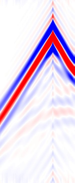
Low frequency extrapolation with deep learning
so the pretrained network can be exposed to the new data col- normal
p distribution centered on zero with the standard devia-
lected on the new model (full-size Marmousi model) with a tion 2/n1 + n2 where n1 are n2 are the numbers of input and
certain generalization level. output units in the weight tensor, respectively. With this ar-
chitecture, we train the network with the Adam optimizer and
5.5
5 use a mini-batch of 20 samples at each iteration. The initial
0.5 4.5
learning rate and forgetting rate of the Adam are the same as
Velocity [km/s]
4
Depth [km]
1 3.5
the original paper (Kingma and Ba, 2014).
3
1.5 2.5
2
2 1.5
0.5 1 1.5 2 2.5 3 -4
Distance [km]
10
MSE
Figure 1: The Marmousi velocity model used to collect the test 10
-6
dataset (unseen during the training process).
10 -8
5.5 10 0 10 1 10 2 10 3
5 epoch
4.5
Velocity [km/s]
4 Figure 3: The training error (MSE) on the Marmousi training
3.5
dataset with the proposed neural network.
3
2.5
2 (a) (b) 10 -3 (c) 10 -3
0.1 5 5
0.5 0.5 0.5
0.05
Figure 2: The nine submodels extracted from the Marmousi 1 1 1
Time [s]
Time [s]
Time [s]
model to collect the training dataset. 1.5 0 1.5 0 1.5 0
2 2 2
-0.05
The acquisition geometry has 30 sources and 300 receivers 2.5 2.5 2.5
evenly spaced on the surface. We use the finite-difference -0.1 -5 -5
1 2 3 1 2 3 1 2 3
modelling method with PML to solve the 2D acoustic wave Distance [km] Distance [km] Distance [km]
equation in the time domain to generate the full-bandwidth
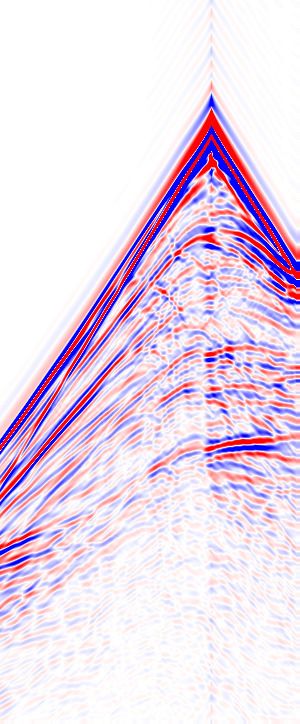
wavefields of both the training and test datasets. The Ricker Figure 4: Comparison between the (a) band-limited recordings
wavelet’s dominant frequency is 20Hz and its maximum am- (5−50Hz), (b) true and (c) predicted low frequency recordings
plitude is one. The sampling interval and the total recording (0.3 − 5Hz). The band-limited data in (a) are the inputs of
time are 1ms and 2.9s, respectively. Each time series or trace CNNs to predict the low frequencies in (b).
is considered as one sample in the dataset, so we have 81, 000
training samples and 9, 000 test samples. For each sample, we The training process of the 500 epochs is shown in Figure 3.
use the data in the band above 5Hz as the inputs and the data in After training, we test the performance of the neural networks
the low frequency band (0.3-5Hz) as the outputs of the neural by feeding the band-limited data in the test set into the model
network. and obtain the extrapolated low frequencies of the full-size
Marmousi model. Figure 4 compares the shot gathers between
The architecture of our neural network is a feed-forward stack the band-limited data (5 − 50Hz), true and extrapolated low
of five sequential combinations of the convolution, batch nor- frequencies (0.3 − 5Hz) where the source is located at the hor-
malization and PReLU layers, and finally followed by one fully izontal distance x = 2.2km. The extrapolated results in Fig-
connected layer which outputs continuous-valued amplitude of ure 4(c) show that the neural networks accurately predict the
the time-domain signal in the low frequency band. The filter recordings in the low frequency band, which are totally miss-
numbers of the five convolutional layers are 128, 64, 128, 64 ing before the test. Figure 5 compares two individual seis-
and 1, respectively. We use only one filter in the last convo- mograms where the receivers are located at the horizontal dis-
lutional layer to reduce the number of channel to one. The tance x = 1.73km and x = 2.25km, respectively. The extrapo-
variation of the channel number can add nonlinearity to our lated low frequency data match the true recordings well. Then
model. The filter size of all the filers in our neural networks we combine the extrapolated low frequencies with the band-
are 80 × 1. Unlike the small filer size commonly used in im- limited data and compare the amplitude spectrum in the fre-
age classification problem, it is essential for bandwidth exten- quency band 0.3 − 20Hz between the data without low fre-
sion to use large filer. The large filter size enables CNNs to quencies, with true low frequencies and with extrapolated low
have enough feasibility to learn the ability of reconstructing frequencies in Figure 6. The pretrained neural networks suc-
the long-wavelength information from the mapping between cessfully recover the low frequency information from the band-
the band-limited data and their true low frequencies. The stride limited data in Figure 6(a). The amplitude spectrum com-
of the convolution is one and the zero padding is used to make parison of the single trace where the receiver is located at
the output length of each convolution layer the same as its in- x = 2.25km (Figure 7) clearly shows that the neural networks
put. The initial value of the bias is zero. The weight initializa- reconstruct the true low frequency energy very well.
tion is via the Glorot uniform initializer (Glorot and Bengio,
2010). It randomly initializes the weights from a truncated Although our method is not based on any physical model, someLow frequency extrapolation with deep learning
limitations can still deteriorate the extrapolation accuracy. The 10 -3 (a)
2
most important limitation is the inevitable generalization error.
Amplitude
As a data-driven statistical optimization method, deep learning 0
requires a large number of samples (usually millions) to be-
come an effective predictor. Since the training dataset in this -2
example is small (81,000 samples) but the model capacity is 0 0.5 1 1.5 2 2.5 3
large (3,290,946 trainable parameters after downsampling the (b)
0.1
signals by factor of three), it is very easy for the neural network
Amplitude
to be overfitting, which seriously constrains the extrapolation 0
accuracy. Therefore, in practice, it is standard to use regular-
ization, dropout or even collect larger training set to relieve -0.1
this problem. In addition, the training time of deep learning is 0 0.5 1 1.5 2 2.5 3
highly related to the size of dataset and the model capacity, and 10 -3 (c)
2
thus is very demanding. For instance, the training process in
Amplitude
this example takes one day on eight GPUs for the 500 epochs. 0
To speed up the training by reducing the number of weights
of neural networks, we can downsample both the inputs and -2
outputs, and then use band-limited interpolation method to re- 0 0.5 1 1.5 2 2.5 3
cover the signal after extrapolation. Another limitation in deep (d)
0.1
learning is due to the unbalanced data. The energy of the direct
Amplitude
wave is very strong compared with the reflected waves, which 0
biases the neural networks towards fitting the direct wave and
having less contribution to the reflected waves. So the extrap- -0.1
olation accuracy of the reflected waves is not as good as the 0 0.5 1 1.5 2 2.5 3
primary wave in this example. Moreover, as we perform band- Time [s]
width extension trace by trace, the accumulation of the pre-
Figure 5: Comparison between the predicted (red line), the true
dicted errors reduce the coherence of the event across traces.
(blue dash line) recording in the low frequency band (0.3 −
Hence, it is probably better to extrapolate multi-trace seismo-
5Hz) and the band-limited recording (black line) (5 − 50Hz)
grams simultaneously. Finally, the effects of the architecture
at the horizontal distance (a) (b) x = 1.73km and (c) (d) x =
and hyperparameters of neural networks on the performance
2.25km.
of bandwidth extension still need to be studied in detail, and
thus we can further improve the extrapolation accuracy by ex- (a) (b) (c)
0 0 0
ploring DNNs that are more suitable.
5 5 5
Frequency [Hz]
Frequency [Hz]
Frequency [Hz]
10 10 10
CONCLUSIONS
15 15 15
In this paper, we have applied deep learning method to the
challenging bandwidth extension problem that is essential for 20
1 2 3
20
1 2 3
20
1 2 3
FWI. We formulate bandwidth extension as a regression prob- Distance [km] Distance [km] Distance [km]
lem in machine learning and propose an end-to-end trainable
Figure 6: Comparison of the amplitude spectrum between (a)
model for low frequency extrapolation. Without any prepro-
the band-limited recordings (5 − 20Hz), the recordings (0.3 −
cessing on the input (the band-limited data) and postprocessing
20Hz) with (b) true and (c) predicted low frequencies (0.3 −
on the output (the extrapolated low frequencies), DNNs have
5Hz).
the ability to recover the low frequencies, which are totally
missing in the seismic data in our experiments. The choice of 80
the architectural parameters is non-unique. The extrapolation
accuracy can be further modified by adjusting the architecture
Amplitude spectrum
60
and hyperparameters of the neural networks.
40
20 with predicted LF
ACKNOWLEDGMENTS with true LF
without LF below 5Hz
0
The authors thank Total SA for support. LD is also supported 0 5 10 15 20
Frequency [Hz]
by AFOSR grant FA9550-17-1-0316, and NSF grant DMS-
1255203. Figure 7: Comparison of the amplitude spectrum at x =
2.25km between the band-limited recording (5 − 20Hz), the
recording (0.3 − 20Hz) with true and predicted low frequen-
cies (0.3 − 5Hz).Low frequency extrapolation with deep learning REFERENCES Araya-Polo, M., T. Dahlke, C. Frogner, C. Zhang, T. Poggio, and D. Hohl, 2017, Automated fault detection without seismic processing: The Leading Edge, 36, 208–214. Araya-Polo, M., J. Jennings, A. Adler, and T. Dahlke, 2018, Deep-learning tomography: The Leading Edge, 37, 58–66. Chen, Y., J. Hill, W. Lei, M. Lefebvre, J. Tromp, E. Bozdag, and D. Komatitsch, 2017, Automated time-window selection based on machine learning for full-waveform inversion: Society of Exploration Geophysicists. De, S., D. Deo, G. Sankaranarayanan, and V. S. Arikatla, 2011, A physics-driven neural networks-based simulation system (phyn- ness) for multimodal interactive virtual environments involving nonlinear deformable objects: Presence, 20, 289–308. Glorot, X., and Y. Bengio, 2010, Understanding the difficulty of training deep feedforward neural networks: Proceedings of the thirteenth international conference on artificial intelligence and statistics, 249–256. Goodfellow, I., Y. Bengio, and A. Courville, 2016, Deep learning, 1. Grzeszczuk, R., D. Terzopoulos, and G. Hinton, 1998, Neuroanimator: Fast neural network emulation and control of physics-based models: Proceedings of the 25th annual conference on Computer graphics and interactive techniques, ACM, 9–20. Guitton, A., H. Wang, and W. Trainor-Guitton, 2017, Statistical imaging of faults in 3d seismic volumes using a machine learning approach: Society of Exploration Geophysicists. He, K., X. Zhang, S. Ren, and J. Sun, 2015, Delving deep into rectifiers: Surpassing human-level performance on imagenet classification: Proceedings of the IEEE international conference on computer vision, 1026–1034. Hornik, K., M. Stinchcombe, and H. White, 1989, Multilayer feedforward networks are universal approximators: Elsevier, 2. Hu, Y., L. Han, Z. Xu, F. Zhang, and J. Zeng, 2017, Adaptive multi-step full waveform inversion based on waveform mode decomposition: Elsevier, 139. Kingma, D. P., and J. Ba, 2014, Adam: A method for stochastic optimization: arXiv preprint arXiv:1412.6980. Lewis, W., and D. Vigh, 2017, Deep learning prior models from seismic images for full-waveform inversion: Society of Exploration Geophysicists. Li, Y. E., and L. Demanet, 2015, Phase and amplitude tracking for seismic event separation: Society of Exploration Geophysicists, 80. ——–, 2016, Full-waveform inversion with extrapolated low-frequency data: Society of Exploration Geophysicists, 81. Richardson, A., 2018, Seismic full-waveform inversion using deep learning tools and techniques: arXiv preprint arXiv:1801.07232. Wang, R., and F. Herrmann, 2016, Frequency down extrapolation with tv norm minimization: Society of Exploration Geophysicists. Wu, R.-S., J. Luo, and B. Wu, 2014, Seismic envelope inversion and modulation signal model: Society of Exploration Geophysi- cists, 79. Zhang, P., L. Han, Z. Xu, F. Zhang, and Y. Wei, 2017, Sparse blind deconvolution based low-frequency seismic data reconstruction for multiscale full waveform inversion: Elsevier, 139.
You can also read