A Novel Unitary ESPRIT Algorithm for Monostatic FDA-MIMO Radar - MDPI
←
→
Page content transcription
If your browser does not render page correctly, please read the page content below
sensors
Article
A Novel Unitary ESPRIT Algorithm for Monostatic
FDA-MIMO Radar
Feilong Liu 1 , Xianpeng Wang 1, *, Mengxing Huang 1, *, Liangtian Wan 2 , Huafei Wang 1            and
Bin Zhang 3
 1    State Key Laboratory of Marine Resource Utilization in South China Sea and School of Information and
      Communication Engineering, Hainan University, Haikou 570228, China; feilongliu@hainu.edu.cn (F.L.);
      wong9525@163.com (H.W.)
 2    Key Laboratory for Ubiquitous Network and Service Software of Liaoning Province, School of Software,
      Dalian University of Technology, Dalian 116620, China; wanliangtian@dlut.edu.cn
 3    Department of Mechanical Engineering, Kanagawa University, 3-27-1 Rokkakubashi, Kanagawa-ku,
      Yokohama 221-8686, Japan; zhangbin@kanagawa-u.ac.jp
 *    Correspondence: wxpeng2016@hainu.edu.cn (X.W.); huangmx09@163.com (M.H.)

 Received: 6 December 2019; Accepted: 31 January 2020; Published: 4 February 2020

 Abstract: A novel unitary estimation of signal parameters via rotational invariance techniques
 (ESPRIT) algorithm, for the joint direction of arrival (DOA) and range estimation in a monostatic
 multiple-input multiple-output (MIMO) radar with a frequency diverse array (FDA), is proposed.
 Firstly, by utilizing the property of Centro-Hermitian of the received data, the extended real-valued
 data is constructed to improve estimation accuracy and reduce computational complexity via unitary
 transformation. Then, to avoid the coupling between the angle and range in the transmitting array
 steering vector, the DOA is estimated by using the rotation invariance of the receiving subarrays.
 Thereafter, an automatic pairing method is applied to estimate the range of the target. Since phase
 ambiguity is caused by the phase periodicity of the transmitting array steering vector, a removal
 method of phase ambiguity is proposed. Finally, the expression of Cramér–Rao Bound (CRB) is
 derived and the computational complexity of the proposed algorithm is compared with the ESPRIT
 algorithm. The effectiveness of the proposed algorithm is verified by simulation results.

 Keywords: Unitary ESPRIT; FDA-MIMO radar; parameter estimation; phase period ambiguity

1. Introduction
     The multiple-input multiple-output (MIMO) radar [1,2], which utilizes multiple antennas to
simultaneously transmit diverse waveforms and receive the reflected signals in similar ways, has
many potential advantages [3]. Unlike the conventional phased-array (PA) radar, MIMO radar has
many superiorities based on its spatial diversity and waveform diversity, such as improving the
system performance with higher degrees-of-freedom (DOFs) [4,5]. Normally, MIMO radar can be
classified into two types based on the spatial location of antenna elements. One is named distributed
MIMO radar, where the transmitting or receiving array elements are placed in different positions,
with a relatively large spacing of elements [6]. The other is the collocated MIMO radar, where both
transmitting and receiving antennas are arranged close to each other [7]. According to whether the
receiver and transmitter are located in the same place, the collocated MIMO radar is further categorized
into the monostatic MIMO radar [8,9] and bistatic MIMO radar [10,11]. A monostatic MIMO radar is
superior in its excellent maneuverability and synchronization between the transmitter and receiver. In
the contemporary defense system, the monostatic radar system is the most mainstream and common
sensor unit in the modern radar network system. A monostatic MIMO radar is addressed in this paper.

Sensors 2020, 20, 827; doi:10.3390/s20030827                                    www.mdpi.com/journal/sensors
Sensors 2020, 20, 827 2 of 17
In radar systems, the target localization is one of the main issues. The angle and range estimation
are the important parts for target localization [12–19]. However, in the beam scanning of both the PA
radar and MIMO radar, the beam pointing is angle-dependent and range-independent. The frequency
diverse array (FDA) radar, in which the direction of focus changes with range, is proposed in [20]. For
the FDA radar, the frequencies of each transmitting array element are different, which can lead to a
range-angle-dependent beampattern [21]. Then, joint angle and range can be estimated simultaneously
in the FDA radar [22–24]. Nevertheless, the resolution of parameter estimation is influenced by the
maximum frequency increment and the array aperture [25]. The maximum number of distinguishable
targets is determined by the number of DOFs and the frequency increment. The range-dependent
beampattern produced by a linear frequency modulation structure is analyzed [26]. In order to estimate
angle and range, a double-pulse method was introduced to obtain the range and angle separately,
where the antenna successively transmits two pulses with non-zero and zero frequency increments [27].
A transmitting subaperture scheme in FDA radar was investigated, where the uniform linear array
(ULA) is divided into multiple overlapping subarrays [28]. To decouple the angle and range, a special
FDA radar with different frequency increments was proposed [29]. A method based on nonuniform
frequency increment was proposed to decouple the FDA beampattern [30]. There are some other
interesting investigations reported in [31–34] about decoupling range and angle in the FDA radar.
In the last few years, FDA-MIMO radar was regarded as a novel radar system combining the
advantages of FDA radar with MIMO radar [35–37]. The FDA-MIMO radar can decouple angle and
range by exploiting the high DOFs of MIMO technique and the angle-range-dependent beampattern
of FDA radar [28,37]. Furthermore, Xu et al. applied a maximum likelihood estimator to obtain
an unambiguous angle and range estimation [38]. The sparse reconstruction-based algorithm was
utilized for the target location with an FDA-MIMO radar [39]. Multiple signal classification (MUSIC)
algorithms were also introduced to the FDA-MIMO radar [40,41]. However, these algorithms with
peak-searching require a large computational complexity. Although a method based on estimation
of signal parameters via rotational invariance techniques (ESPRIT) algorithm has been introduced to
obtain the range and angle estimation and reduce the complexity [42], there are still some challenges,
such as a low estimation performance, high complexity and phase ambiguity.
In this paper, an improved unitary ESPRIT method for angle and range estimation in monostatic
FDA-MIMO radar is presented. Then, a method is proposed to achieve the automatic pairing of
angle and range. The reason for phase ambiguity is analyzed, and a simple and efficient solution is
proposed. The Cramér–Rao Bound (CRB) for target parameter of monostatic FDA-MIMO radar is
derived. Computational complexity analysis is provided to be compared with that of [42].
The paper is summarized as follows. Section 2 introduces the signal model of the monostatic FDA
radar. We propose an improved unitary ESPRIT algorithm with an automatic pairing, and investigate
a phase judgment in Section 3. In Section 4, we derive the CRB of the monostatic FDA-MIMO radar
and offer the specific analysis of computational complexity. Several simulation results are provided
to indicate the effectiveness of the presented algorithm in Section 5. The conclusion of the paper is
indicated in Section 6.
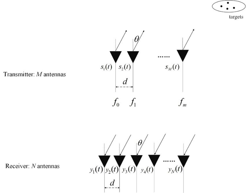
2. Signal Model of Monostatic FDA-MIMO Radar
The signal model of monostatic FDA-MIMO radar is shown in Figure 1, which is configured
with M-antenna-transmitting ULA and N-antenna-receiving ULA. The transmitting and receiving
arrays are placed together to guarantee that the DOA is the same as the direction of departure (DOD).
The element interval of the transmitting array is equal to that of receiving array, and they are both
marked with d. The element interval d is set to half of the maximal wavelength. The first element
of transmitting array is assumed as the reference. The frequency of the m-th signal emitted by the
transmitting array is calculated by
fm = f0 + (m − 1)∆ f , m= 1, 2, · · · , m (1)Sensors 2020, 20, 827 3 of 17 where f 0 is the referenced frequency, and ∆f is the deviation of adjacent transmitting frequencies, where ∆f
Sensors 2020, 20, 827 4 of 17
Sensors 2020, 20, x FOR PEER REVIEW 4 of 18
Figure
Figure 1.
1. Monostatic
MonostaticFDA-MIMO
FDA-MIMOradar.
radar.
3. Unitary
3. UnitaryESPRIT
ESPRITAlgorithm
Algorithmfor
for Ange
Ange and
and Range
Range Estimation
Estimation
3.1. Rotation
3.1. RotationInvariance
Invarianceof
of Subarrays
Subarrays
In this
In this section,
section, the
the complex-valued
complex-valued rotation
rotation invariance
invariance relation
relation is
is introduced
introduced withwith respect
respect to
to the
the
transmitting array and receiving array, respectively. As shown in Figure 2, the transmitting
transmitting array and receiving array, respectively. As shown in Figure 2, the transmitting array and array
and receiving
receiving arrayarray of monostatic
of monostatic FDA-MIMO
FDA-MIMO radar
radar areare dividedinto
divided intotwo twooverlapping
overlapping subarrays,.
subarrays,.
Assuming that
Assuming that the
the two
two adjacent
adjacent subarrays
subarrays are
are identical,
identical, there
there exists
exists aa rotation
rotation invariance
invariance between
between
Subarray 1 and Subarray 2, or Subarray 3 and Subarray 4. According
Subarray 1 and Subarray 2, or Subarray 3 and Subarray 4. According to Equation (4), due toto Equation (4), due to the
the
existence of a coupling relationship between DOA and the range, it is necessary
existence of a coupling relationship between DOA and the range, it is necessary to obtain DOA to obtain DOA
information by
information by the
the rotation
rotation invariance
invariance relationship
relationship ofof the
the receiving
receiving subarrays,
subarrays, andand substitute
substitute the
the
estimated DOA into the rotation invariance of transmitting arrays to get the range
estimated DOA into the rotation invariance of transmitting arrays to get the range information. The information. The
complex-valued invariance
complex-valued invariance relationship
relationship of
of the
the Subarray
Subarray 33 and
and Subarray
Subarray 44 can can be
be expressed
expressed asas [42]
[42]
π sinθθk
J2 b(Jθ2b
k )(θ=
k
e jπe jsin
)= JJ11b((θθk k)) (12)
(12)
where = [[I NIN−1
where JJ11 = −1
] )and
0(N − 1)0×(1N−1 ×1 ] and
J 2 = [J02 (N= [ 0I(N−1
− 1) × 1
] areIselection
N − 1 )×1 N−1 ] are matrices,
selection and 0w denotes
matrices, and 0the w × w null
w denotes the
w × w null matrix. The functions
matrix. The functions of J1 and J2 are to of J and J are to select the first and last
1 select2 the first and last N − 1 rows of a matrix, respectively. N − 1 rows of a matrix,
Based on Equation (12), the invariance the
respectively. Based on Equation (12), invariance
relationship in relationship
the joint steering in thevector
joint can
steering vector can
be expressed as be
expressed as
jπ sinθ
( IM ⊗ J2 ⊗
(IM )c(Jr2k),cθ (rkk ),θ=
k
) =e jπe sin θkk (IM
M
⊗
⊗ J11 )cc((rrk k,θ, θ))
k k
(13)
(13)
Underthe
Under theassumption ofKKtargets,
assumptionof targets,the therotation
rotationinvariance
invarianceof ofeach each target
target can
can be
be written
written into
into aa
matrix form
matrix form
(IM ⊗ J2 )C = (IM ⊗ J1 )CΞR (14)
(IM ⊗ J )C
2 θ1
= (I ⊗ J ) C Ξ (14)
e jπ sin M R
1
.
ΞR = .. (15)
e jπ sin θ1
jπ sin θ
e
k
ΞR = (15)
e jπ sin θk
Sensors 2020, 20, 827 5 of 17
where ΞR contains the angle information of all targets. It can be shown that the columns in C span the
same signal subspace as the column vectors in the signal subspace Es [43], we can obtain the following
relationship
ES = CΘ (16)
where Es is composed of the K eigenvectors corresponding to the largest K eigenvalues of the covariance
matrix of Y, and Θ is a non-singular matrix. Substituting Equation (16) into Equation (14), we can
obtain the relationship between signal space of the subarrays
(IM ⊗ J2 )ES = (IM ⊗ J1 )ES ΨR (17)
−1
where ΨR =
Sensors 2020, 20,Θ
x FORΞRPEER
Θ. ItREVIEW
can be noticed that the diagonal elements of ΞR are the eigenvalues of Ψ R . 18
6 of
Figure 2. The
Figure 2. The division
division of
of the
the transmitting
transmitting array
array and
and receiving array.
receiving array.
3.2. Unitary ESPRIT
Next, the in FDA-MIMO
complex-valued Radar
rotation invariance between Subarray 1 and Subarray 2 is considered
to estimate range. aThe
In this section, transmitting invariance
complex-valued steering vectors of Subarray
is transformed into 1a and Subarray
real-valued 2 satisfy and
invariance, the
following equation
the DOAs and ranges are estimated by using the unitary ESPRIT algorithm. As there is no central
∆f
J4 a(rk , in
Hermitian symmetric characteristic θk )Y,=an e j(πextended
sin θk −4π c rk )
J3 a(rk , θdata
receiving k) matrix with the symmetric(18)
structure is defined as [44,45]
where J3 = [ IM−1 0(m−1)×1 ] and J4 = [ 0(m−1)×1 IM−1 ] stand for selection matrices to select the
first and last M − 1 rows, respectively. For K = Y Πthis
Z targets, MN
ΠL
Y *relationship is extended to the joint steering
(22)
vector which can be expressed as
where ΠMN is an M × N exchange matrix with ones on its anti-diagonal and zeros elsewhere. Over the
(IN ⊗ J4 )C =Centro-Hermitian
construction of Equation (22), Z is a generalized (IN ⊗ J3 )CΞT matrix. The complex matrix (19) Z is
transformed into the real-valued matrix Г by utilizing ∆f
the unitary transformation.
It can be expressed
as [43] e j(π sin θ1 −4π c r1 )
ΞT =
. .
(20)
Γ = Q ZQ = Q Y Π Y Π Q
H H . *
MN L ∆2fL (23)
MN 2L MN
e j(π sin θK −4π c rK )
where (.)H represents the conjugate transpose operator, and the sparse unitary matrix Qw is defined
where ΞT contains the ranges of all the targets. According to Equation (16), Equation (19) can be
as
rewritten as
(IN ⊗1 J4 )IEw S = j(IIwN ⊗ J3 )ES ΨT (21)
Qw = Π w is even
−
2 w of the wcovariance
jΠ
where ΨT = Θ−1 ΞT Θ. Because the calculation matrix of Y and the acquisition of ES
are based on complex-valued data, DOAs and I w ranges0 jIare estimated with relatively high complexity.
(24)
w
Hence, based on the idea of a unitary 1 Talgorithm,Ta novel
ESPRIT w is odd
unitary ESPRIT algorithm is proposed
Qw = 0 2 0
to reduce complexity and improve estimation 2 accuracy.
Π
w
0 − jΠ w
Compared with Equation (9), Equation (22) is competent in doubling the number of snapshots. Then,
the real-valued covariance RГ of the extended received data can be acquired by using the maximum
likelihood estimationSensors 2020, 20, 827 6 of 17
3.2. Unitary ESPRIT in FDA-MIMO Radar
In this section, a complex-valued invariance is transformed into a real-valued invariance, and
the DOAs and ranges are estimated by using the unitary ESPRIT algorithm. As there is no central
Hermitian symmetric characteristic in Y, an extended receiving data matrix with the symmetric
structure is defined as [44,45] h i
Z = Y ΠMN Y∗ ΠL (22)
where ΠMN is an M × N exchange matrix with ones on its anti-diagonal and zeros elsewhere. Over the
construction of Equation (22), Z is a generalized Centro-Hermitian matrix. The complex matrix Z is
transformed into the real-valued matrix Γ by utilizing the unitary transformation. It can be expressed
as [43] h i
Γ = QH MN ZQ 2L = Q H
MN Y Π MN Y ∗ Π Q
L 2L (23)
where (.)H represents the conjugate transpose operator, and the sparse unitary matrix Qw is defined as
" #
Iw jIw
√1
Qw =
Πw
2 −jΠw w is even
Iw 0 jIw (24)
√
√1 0T 0T
Qw = 2 w is odd
2
Πw
0 − jΠw
Compared with Equation (9), Equation (22) is competent in doubling the number of snapshots. Then,
the real-valued covariance RΓ of the extended received data can be acquired by using the maximum
likelihood estimation
RΓ = 2L 1
ΓΓ
H
= 12 QH R Q (25)
h MN Z MN i
= 2 QMN RY + ΠMN RY ΠMN QMN
1 H ∗
where RY and RZ are the covariance calculated by Y and Z, respectively. The signal subspace ÊS
corresponds to K eigenvectors of large eigenvalues of RΓ . The remaining MN − K eigenvectors of small
eigenvalues can obtain the noise subspace ÊN . Hence, ÊS and ÊN are both real-valued. Due to the
unitary transformation in Equation (23), the complex-valued invariance relation in Equation (13) is
transformed into real-valued invariance relation as follows
π sin θk
K2 dk = tan K1 dk (26)
2
K1 = Re QH (
(N−1)m M
I ⊗ J 2 ) Q MN (27)
K2 = Im QH (
(N−1)m M
I ⊗ J 2 ) Q MN (28)
where dk = QH c is the real-valued steering vector. Re{.} and Im{.} denote the real and imaginary parts
MN k
of a complex number, respectively. Considering K-independent targets, Equation (26) is expressed as
K2 D = K1 DΦR (29)
π sin θ
tan( 2 1 )
..
ΦR = (30)
.
π sin θ
tan( 2 k )
Sensors 2020, 20, 827 7 of 17
where D = [d1 , d2 , . . . , dk ], and ΦR is a real diagonal matrix whose diagonal elements contain the
desired angle information. According to Equation (16), Equation (29) can be rewritten as
K2 ÊS = K1 ÊS ΣR (31)
where ΣR = Θ−1R ΦR ΘR . ΘR is the left eigenvector matrix of ΣR . By using the total least squares (TLS)
method to solve Equation (31), DOA can be estimated as follows
2arctan[(ΦR )]k
!
θ̂k = arcsin (32)
π
Similarly, the rotation invariance between Subarray 1 and Subarray 2 can be transformed into
r
π(sin θk − 4∆ f ck )
K4 dk = tan K3 dk (33)
2
K3 = Re QH (
(m−1)N N
I ⊗ J 4 ) Q MN (34)
K4 = Im QH (
(m−1)N N
I ⊗ J 4 ) Q MN (35)
For K targets, Equation (33) can be integrated into matrix form
K4 D = K3 DΦT (36)
r1
tan( π sin θ1 −4π∆ f c )
2
..
ΦT = .
(37)
rk
π sin θk −4π∆ f c
tan( 2 )
where ΦT is a real diagonal matrix whose diagonal elements contain the desired range of information.
In the same way as Equation (31), we can obtain the rotational invariance of the signal subspace
K4 ÊS = K3 ÊS ΣT (38)
where ΣT = Θ−1T ΦT ΘT . ΘT is the inverse of the left eigenvector matrix of ΣT . Substituting Equation (32)
into Equation (37), the range estimation is solved with the TLS method.
2arctan[(ΦR )]k − 2arctan[(ΦT )]k
r̂k = c (39)
4π∆ f
Due to the correlation of ΦR and ΦT in Equation (39), the ranges will be miscalculated without the
pairing of ΦR and ΦT . Hence, we employ an automatic pairing method to implement correct range
estimation.
3.3. The Pairing of DOAs and Ranges
In this section, we analyze the speciality of ΘT and ΘR , and introduce the means to achieve pairing.
ΘT and ΘR are eigenvectors of ΣT and ΣR , respectively. Since ΣT and ΣR are calculated by ÊS , there
must be a random row of ΘR identical to a specific row of ΘT . Supposing that all of the K targets are
independent, we notice that any two rows of ΘR are orthogonal because any two eigenvalues of ΘT
are different. In this paper, considering algorithm complexity, we obtain the automatic pairing of ΦT
and ΦR by decomposing the ΣT + jΣR , which can be expressed as
ΣT + jΣR = Θ−1
TR ΦT + jΦR ΘTR
(40)Sensors 2020, 20, 827 8 of 17
where ΘTR is the left eigenvector matrix. Hence, ΦT and ΦR can be automatically paired by the
eigenvector matrix ΘTR . Considering the periodic phase ambiguity problem, we take a step to
distinguish the phase ambiguity before calculating ranges.
3.4. The Solution of Periodic Ambiguity of Transmitter
In this section, we analyze the periodic phase ambiguity and adopt an ambiguity judgment
method to obtain the correct range estimation. Since the period of tan in Equation (26) is π, and sinθk
∈ (−1, 1), DOAs can be estimated by Equation (32) without periodic ambiguity. However, there is
phase ambiguity in range estimation due to sinθk − 4∆frk /c ∈ (−3, 1) and rk ∈ (0, c/2∆f ). Therefore, rk
obtained by Equation (39) is misestimated, because the tangent of π(sinθk − 4∆frk /c)/2 is equal to the
tangent of π(sinθk − 4∆frk /c)/2 + π when sinθk − 4∆frk /c ∈ (−3, −1). Note that π(sinθk − 4∆frk /c)/2 <
πsinθk /2< π(sinθk − 4∆frk /c)/2 + π. Since ΦT and ΦR are relevant to π(sinθk − 4∆frk /c)/2 and πsinθk /2,
respectively, we determine the range of π(sinθk − 4∆frk /c)/2 by comparing arctan[ΦT ]k and arctan[ΦR ]k .
If arctan[ΦT ]k > arctan[(ΦR )]k , due to arctan[ΦT ]k ∈ (−π/2, π/2), there is a phase ambiguity, as π(sinθk −
4∆frk /c)/2 is considered to lie in (−π/2, π/2) when π(sinθk − 4∆frk /c)/2 ∈ (−3π/2, −π/2). We can use a
phase shift π to solve the periodic phase ambiguity problem. Hence, the true phase value of ΦT can be
calculated as
π
(sin θ̂k − 4∆ f rk /c) = arctan(ΦT ) − π (41)
2
rk can be given by
arctan[(ΦR )]k − arctan[(ΦT )]k + π
r̂k = c (42)
2π∆ f
Otherwise, there is no phase ambiguity and the true phase value of ΦT can be given by
π
(sin θ̂k − 4∆ f rk /c) = arctan(ΦT ) (43)
2
rk can be given by
arctan[(ΦR )]k − arctan[(ΦT )]k
r̂k = c (44)
2π∆ f
The main steps of the proposed algorithm are summarized in Algorithm 1.
Algorithm 1: A Novel Unitary ESPRIT for Monostatic FDA-MIMO Radar
1: Construct the extended received data matrix Z via (22).
2: Take the unitary transformation using (23) and obtain RΓ via (25).
3: Perform eigenvalue decomposition of RΓ and return ÊS .
4: Calculate ΣT and ΣR via (31) and (38), respectively.
5: Obtain the automatically paired ΦT and ΦR via (40).
6: Compute the DOAs by (32) and ranges by (42) or (44).
4. CRB and Complexity Analysis
4.1. CRB
In this section, we analyze the CRBs of angle and range for the monostatic FDA-MIMO radar.
According to Equation (9), the concrete expression of RY is written as
1 H
RY = YY = CRH CH + σ2 I (45)
LSensors 2020, 20, 827 9 of 17
where RH is the covariance of H in Equation (9), and L is the number of snapshots, and σ2 denotes the
noise power. Under the assumption of K targets, the unknown parameter to be estimated is
T
η = [θT , rT ] = [θ1 , . . . , θk , r1 , . . . , rk ]T (46)
Then, the Fisher information matrix (FIM), with respect to η, is [41]
" #
Fθθ Fθr
F= (47)
Frθ Frr
The expression of every block of F can be written as
2L
T
H ⊥ H −1
Fθθ = Re C Π
θ C C θ R H C R CR H (48)
σ2 Y
2L
T
Fθr = 2 Re CH Π
θ C
⊥
C r RH C H −1
R CRH (49)
σ Y
2L
T
Frθ = 2 Re CH r Π ⊥
C
C θ R H CH −1
R CR H (50)
σ Y
2L
T
H ⊥ H −1
Frr = 2 Re Cr ΠC Cr RH C RY CRH (51)
σ
−1
where Cθ and Cr are partial derivations of C with respect to θ and r, and Π⊥
C = I − C CHC CH . The
Cθ and Cr can be written as
Cθ = [c1θ , c2θ , . . . , cKθ ] (52)
Cr = [c1r , c2r , . . . , cKr ] (53)
where
∂c(θk , rk ) ∂a(θk , rk ) ∂b(θk )
ckθ = = ⊗ b(θk ) + a(θk , rk ) ⊗ k = 1, 2, . . . K (54)
∂θk ∂θk ∂θk
∂c(θk , rk ) ∂a(θk , rk )
ckr = = ⊗ b(θk ), k = 1, 2, . . . K (55)
∂rk ∂rk
We derive part of Equations (54) and (55) as
0
∂a(θk , rk )
= jπ cos(θk )
.. a(θk , rk )
(56)
.
∂θk
M−1
0
∂b(θk )
= jπ cos(θk )
.. b(θk )
(57)
.
∂θk
N−1
and
0
∂a(θk , rk ) ∆ f
= −j4π .. a(θk , rk )
(58)
.
∂rk c
M−1
Then, every block of F is determined by Equations (48)–(51). Then, the CRB matrix can be obtained by
σ2 n H ⊥ o−1
CRB = F−1 = Re W ΠC W PT (59)
2LSensors 2020, 20, 827 10 of 17
" #
P1 P2
where W = [Cθ Cr ], P = and P1 = P2 = P3 = P4 = RH CH R−1
Y
CRH .
P3 P4
4.2. Complexity
To compare the presented algorithm and the ESPRIT algorithm of [42], the specific analysis
of the computational complexity is provided. In this paper, we transform received data from the
complex domain to the real domain by a unitary transformation. Hence, the calculation of eigenvalue
decomposition and generalized inverse depend on the real domain. The calculation of a complex
product is equivalent to the calculation of four real products. The concentration of computational
complexity in the presented algorithm is based on calculating the covariance matrix, utilizing the
eigenvalue decomposition, obtaining signal subspace, solving the solution for angle and range, and
achieving pairing for angle and range. The calculation of RΓ needs O{2L(MN)2 } flops, where M and N
denote the number of transmitting and receiving array elements, respectively, and L is the number of
snapshots. The eigenvalue decomposition of RΓ , to obtain the signal subspace and the noise subspace,
needs O{(MN)3 } flops. The complexity required to solve for ΣR is O{M(N − 1)(2K)2 }, where K is the
number of targets. Similarly, solving ΣT needs O{N(M − 1)(2K)2 } flops. The eigenvalue decomposition
in Equation (40) and the pairing of angle and range need O{4(2K)3 + 2K3 }. Here, we ignore the
complexity of solving periodic ambiguity steps because they are too small. Thus, the complexity of the
proposed algorithm is
O 2L(MN )2 + (MN )3 + 4K2 (2MN − m − N ) + 34K3
n o
(60)
In [42], the complexity of the ESPRIT algorithm for estimation of angle and range is
O 2L(MN )2 + (2MN )3 + 4K2 (5MN − 2m − 2N ) + 31K3
n o
(61)
By the comparison of Equations (60) and (61), the computational complexity of the proposed algorithm
is much lower than [42]. Furthermore, later in the simulation, we give the comparison results regarding
complexity.
5. Simulation Results
In this section, we provide several simulation results to evaluate the performance of the proposed
algorithm for angle and range estimation in monostatic FDA-MIMO radar with ULA. The ESPRIT
algorithm in the same model is chosen for comparison [42]. In all simulations, assume that the reference
carrier frequency f 0 , namely the minimum frequency, is 3 GHz, and the frequency increment ∆f is
103 Hz. According to the relationship of Equation (1), the maximum frequency and the number of
bins depend on the number of transmitting arrays. The noise is assumed to be the uniform complex
white Gaussian noise. The reflection coefficient of the target is set to 1. The number of Monte Carlo
experiments is set to 500.
5.1. Estimated Results
In this section, the SNR is set to 10 dB, and the number of snapshots is 50, and the number of
transmitting array elements M and receiving array elements N are both set to eight. Figure 3a,b shows
the unpaired and paired estimation of range, respectively, obtained by the proposed algorithm, where
the two-dimensional parameters of the target are set to (45◦ , 40 km) and (30◦ , 10 km). It is noted that
an incorrect range estimation is shown in Figure 3a, which is caused by the mismatch between the
eigenvalues of ΣR and ΣT . It is seen in Figure 3b that the pairing method can obtain the correct range
estimation. Figure 4a,b shows the estimation results of angle and range acquired by the proposed
algorithm and the ESPRIT algorithm, where the targets in Figure 4a are the same as those of Figure 3,
and the targets in Figure 4b are assumed to be (45◦ , 40 km) and (−30◦ , 70 km). As there is no periodSensors 2020, 20, 827 11 of 17
ambiguity for (45◦ , 40 km) and (30◦ , 10 km), the proposed algorithm and the ESPRIT algorithm can
both obtain accurate estimation, as shown in Figure 4a. It is shown in Figure 4b that the proposed
algorithm can effectively solve the period ambiguity, because (−30◦ , 70 km) satisfies sinθk − 4∆frk /c ∈
(−3, −1).
Sensors 2020, 20, x FOR PEER REVIEW 12 of 18
(a)
(b)
Figure3.3.The
Figure The range
range estimation
estimation results
results obtained
obtained by thebyproposed
the proposed algorithm
algorithm with unpairing
with unpairing and
and pairing.
pairing. (a) Unpaired range estimation; (b) paired range
(a) Unpaired range estimation; (b) paired range estimation. estimation.
5.2. RMSE Versus SNR
In this section, the target is set to (45◦ , 40 km) and (30◦ , 10 km), and the number of snapshots is 50.
The number of transmitting array elements M and receiving array elements N are set to M = N = 4 and
M = N = 8, respectively. The SNR increases from 0 dB to 20 dB, with each step being 2 dB. Figure 5a,b
shows the root mean square errors (RMSEs) of the proposed algorithm and the ESPRIT algorithm with
the different SNR. Meanwhile, the CRBs of angle and range in the monostatic FDA-MIMO radar are(a)
Sensors 2020, 20, 827 12 of 17
chosen for the assessment of the performance of the proposed algorithm. The RMSEs of angle and
range are respectively defined as
v
u
G K
u
t
1 1XX 2
RMSEθ = (θk − θ̂k ) (62)
GK
g=1 k =1
v
u
G K
u
t
1 1XX
RMSEr = (rk − r̂k )2 (63)
GK
g=1 k =1
(b)
where G represents the number of Monte Carlo experiments. We can observe that the RMSEs of the
proposed algorithm are closer to the CRBs. This indicates that the performance of the proposed method
Figure 3. The range estimation results obtained by the proposed algorithm with unpairing and
is better than theUnpaired
pairing. (a) ESPRIT range
algorithm with the
estimation; identical
(b) paired SNR.
range estimation.
Sensors 2020, 20, x FOR PEER REVIEW (a) 13 of 18
(b)
Figure4.4.Location
Figure Locationofofthe
thetarget
targetunder
underdifferent
differenttarget
targetparameters
parametersbybythetheproposed
proposedalgorithm
algorithmand
and
ESPRIT algorithm. (a) Targets without phase ambiguity; (b) targets with phase ambiguity.
ESPRIT algorithm. (a) Targets without phase ambiguity; (b) targets with phase ambiguity.
5.2. RMSE Versus SNR
In this section, the target is set to (45°, 40 km) and (30°, 10 km), and the number of snapshots is
50. The number of transmitting array elements M and receiving array elements N are set to M = N =
4 and M = N = 8, respectively. The SNR increases from 0 dB to 20 dB, with each step being 2 dB. Figure
5a,b shows the root mean square errors (RMSEs) of the proposed algorithm and the ESPRIT algorithm1 1 G K
RMSEr = (r − rˆ )2
G K g =1 k = 1 k k
(63)
where G represents the number of Monte Carlo experiments. We can observe that the RMSEs of the
Sensors 2020, 20, 827 13 of 17
proposed algorithm are closer to the CRBs. This indicates that the performance of the proposed
method is better than the ESPRIT algorithm with the identical SNR.
10 1
ESPRIT(M=N=8)
Unitary ESPRIT(M=N=8)
CRB(M=N=8)
ESPRIT(M=N=4)
Unitary ESPRIT(M=N=4)
CRB(M=N=4)
10 0
10 -1
10 -2
0 2 4 6 8 10 12 14 16 18 20
SNR (dB)
Sensors 2020, 20, x FOR PEER REVIEW 14 of 18
(a)
10 4
ESPRIT(M=N=8)
Unitary ESPRIT(M=N=8)
CRB(M=N=8)
ESPRIT(M=N=4)
Unitary ESPRIT(M=N=4)
CRB(M=N=4)
10 3
10 2
10 1
0 2 4 6 8 10 12 14 16 18 20
SNR (dB)
(b)
Figure5.5.Estimation
Figure Estimationof
oftarget
targetparameters
parametersby
bythe
theproposed
proposedalgorithm
algorithmand
andESPRIT
ESPRITalgorithm
algorithmwith
with
different SNR. (a) RMSE of DOA versus SNR; (b) RMSE of range versus
different SNR. (a) RMSE of DOA versus SNR; (b) RMSE of range versus SNR. SNR.
5.3.
5.3.RMSE
RMSEVersus
VersusNumber
NumberofofSnapshots
Snapshots
InInthe ◦ , 40 km) and (30◦ , 10 km), and the SNR is 0 dB. The
thesimulation,
simulation,thethetarget
targetisisset
settoto(45
(45°, 40 km) and (30°, 10 km), and the SNR is 0 dB. The
number of transmitting array elements M and
number of transmitting array elements M and receiving receiving array elements
array N areNboth
elements set toset
are both eight and four,
to eight and
respectively. We set We
four, respectively. the initial
set thenumber
initial of snapshots
number to be 50, and
of snapshots observe
to be theobserve
50, and effect ofthe
theeffect
number of
of the
snapshots
number ofonsnapshots
the RMSEs onby intervals
the RMSEs of by100. Figureof6a,
intervals b shows
100. Figurethe
6a,RMSEs
b showsof the
angle and range
RMSEs versus
of angle and
the number
range versusof snapshots,
the number respectively. This respectively.
of snapshots, indicates thatThisthe performance of the
indicates that the proposed
performancealgorithm
of the
isproposed
better than that of the
algorithm ESPRIT
is better algorithm
than with
that of the the same
ESPRIT numberwith
algorithm of snapshots.
the same number of snapshots.
5.4. Computational Complexity101
ESPRIT(M=N=8)
In this part, the runtime of the proposed algorithm is compared with that of the ESPRIT algorithm.
Unitary ESPRIT(M=N=8)
CRB(M=N=8)
◦ ◦
The target is set to (45 , 40 km), and (30 , 10 km), the SNR isESPRIT(M=N=4)
set to 0 dB, and the number of snapshots
Unitary ESPRIT(M=N=4)
is 50. The number of transmitting
10 0
array elements is equal to that of the receiving array elements, i.e.,
CRB(M=N=4)
M = N, and the transmitting array number M is changed in this simulation. The required runtime of
the two algorithms is shown in Figure 7. The runtime of the proposed algorithm is less than that of the
ESPRIT algorithm.
10 -1
10 -2
50 100 150 200 250 300 350 400 450 500 550
Number of Snapshots
(a)In the simulation, the target is set to (45°, 40 km) and (30°, 10 km), and the SNR is 0 dB. The
number of transmitting array elements M and receiving array elements N are both set to eight and
four, respectively. We set the initial number of snapshots to be 50, and observe the effect of the
number of snapshots on the RMSEs by intervals of 100. Figure 6a, b shows the RMSEs of angle and
range2020,
Sensors versus
20, 827the number of snapshots, respectively. This indicates that the performance 14ofofthe
17
proposed algorithm is better than that of the ESPRIT algorithm with the same number of snapshots.
10 1
ESPRIT(M=N=8)
Unitary ESPRIT(M=N=8)
CRB(M=N=8)
ESPRIT(M=N=4)
Unitary ESPRIT(M=N=4)
CRB(M=N=4)
10 0
10 -1
10 -2
50 100 150 200 250 300 350 400 450 500 550
Number of Snapshots
(a)
Sensors 2020, 20, x FOR PEER REVIEW 15 of 18
RMSE (m)
Figure 6. Estimation of target parameters by the proposed algorithm and ESPRIT algorithm with
different SNR. (a) RMSE of DOA versus SNR; (b) RMSE of range versus SNR.
5.4. Computational Complexity
In this part, the runtime of the proposed algorithm is compared with that of the ESPRIT
algorithm. The target is set to (45°, 40 km), and (30°, 10 km), the SNR is set to 0 dB, and the number
of snapshots is 50. The number of transmitting array (b) elements is equal to that of the receiving array
elements, i.e., M = N, and the transmitting array number M is changed in this simulation. The required
Estimation
Figureof6.the
runtime of target is
two algorithms parameters
shown inby the proposed
Figure algorithmofand
7. The runtime theESPRIT algorithm
proposed with is less
algorithm
different SNR. (a) RMSE of DOA
than that of the ESPRIT algorithm. versus SNR; (b) RMSE of range versus SNR.
10 -1
ESPRIT
The proposed
10 -2
10 -3
8 10 12 14 16 18 20
Number of Array Elements
Figure7.7.The
Figure Theruntime
runtimeofofthe
theESPRIT
ESPRITalgorithm
algorithmand
andthe
theproposed
proposedalgorithm
algorithmwith
withthe
thedifferent
differentnumber
number
ofofarray
arrayelements.
elements.
We can summarize this with two situations, according to the existence of periodic ambiguity. In
the case of periodic ambiguity, the ESPRIT algorithm cannot obtain the correct estimation of target
parameters, but the proposed algorithm can accurately get the angles and ranges of the target. In the
absence of periodic ambiguity, the proposed algorithm and ESPRIT algorithm can both obtain a
correct estimation of target parameters. The estimation accuracy of the proposed algorithm is higherSensors 2020, 20, 827 15 of 17
We can summarize this with two situations, according to the existence of periodic ambiguity. In
the case of periodic ambiguity, the ESPRIT algorithm cannot obtain the correct estimation of target
parameters, but the proposed algorithm can accurately get the angles and ranges of the target. In the
absence of periodic ambiguity, the proposed algorithm and ESPRIT algorithm can both obtain a correct
estimation of target parameters. The estimation accuracy of the proposed algorithm is higher than that
of the ESPRIT algorithm, and the running time is shorter than that of the ESPRIT algorithm. Due to
the extended receiving data and the unitary transformation operation of the proposed algorithm, the
number of snapshots is as twice as the original number, and the complex data is transformed into the
real data, which greatly reduces the computational complexity.
6. Conclusions
In this paper, a novel unitary ESPRIT algorithm is proposed for the angle and range estimation in
a monostatic FDA-MIMO radar. In the proposed method, the angle and range are estimated by using
the rotation invariance between the specific subarrays. Then, we make a specific analysis of periodic
ambiguity and propose a method to solve that. Additionally, the computational complexity of the
proposed algorithm is compared with that of the ESPRIT algorithm. The theoretical performance of
the proposed algorithm is verified by computer simulation. In future work, we will focus on how to
estimate the parameters of targets when mutual coupling errors exist in the FDA-MIMO radar, how to
use the proposed algorithm in more general array structures, and how to use the proposed algorithm
to estimate parameters in a colored noise environment.
Author Contributions: F.L. wrote the paper. X.W. and M.H. proposed the original idea. L.W. designed the
simulations and analyzed the data, and H.W. and B.Z. checked the paper. All authors have read and agreed to the
published version of the manuscript.
Funding: This work was funded by Key Research and Development Program of Hainan Province (No.
ZDYF2019011), the National Natural Science Foundation of China (No. 61701144, No. 61861015, No. 61961013), the
Program of Hainan Association for Science and Technology Plans to Youth R&D Innovation (No. QCXM201706),
the scientific research projects of University in Hainan Province (No. Hnky2018ZD-4), Young Elite Scientists
Sponsorship Program by CAST (No. 2018QNRC001), Collaborative Innovation Fund of Tianjin University and
Hainan University (No. HDTDU201906), the Scientific Research Setup Fund of Hainan University (No. KYQD
(ZR) 1731), and the Graduate Innovation Research Project of Hainan Province (No. Hys2019-25).
Conflicts of Interest: The authors declare no conflict of interest.
References
1. Bliss, D.W.; Forsythe, K.W. Multiple-input multiple-output (MIMO) radar and imaging: Degrees of
freedom and resolution. In Proceedings of the 37th Asilomar Conference Signals, Systems, and Computers
(ASILOMAR 2003), Pacific Grove, CA, USA, 9–12 November 2003; pp. 54–59.
2. Fishler, E.; Haimovich, A.; Blum, R.; Chizhik, D.; Cimini, L.; Valenzuela, R. MIMO radar: An idea whose time
has come. In Proceedings of the IEEE Radar Conference, Philadelphia, PA, USA, 26–29 April 2004; pp. 71–78.
3. Wan, L.; Kong, X.; Xia, F. Joint Range-Doppler-Angle Estimation for Intelligent Tracking of Moving Aerial
Targets. IEEE Internet Things J. 2018, 5, 1625–1636. [CrossRef]
4. Huang, H.; Song, Y.; Yang, J.; Gui, G.; Adachi, F. Deep-Learning-Based Millimeter-Wave Massive MIMO for
Hybrid Precoding. IEEE Trans. Veh. Technol. 2019, 68, 3027–3032. [CrossRef]
5. Huang, H.; Yang, J.; Huang, H.; Song, Y.; Gui, G. Deep Learning for Super-Resolution Channel Estimation
and DOA Estimation Based Massive MIMO System. IEEE Trans. Veh. Technol. 2018, 67, 8549–8560. [CrossRef]
6. Haimovich, A.M.; Blum, R.S.; Cimini, L.J. MIMO radar with widely separated antennas. IEEE Signal Process.
Mag. 2008, 25, 116–129. [CrossRef]
7. Li, J.; Stoica, P. MIMO radar with colocated antennas. IEEE Signal Process. Mag. 2007, 24, 106–114. [CrossRef]
8. Xie, R.; Liu, Z.; Zhang, Z. DOA estimation for monostatic MIMO radar using polynomial rooting. Signal
Process. 2010, 90, 3284–3288. [CrossRef]
9. Wang, X.; Wang, W.; Liu, J.; Li, X.; Wang, J. A sparse representation scheme for angle estimation in monostatic
MIMO radar. Signal Process. 2014, 104, 258–263. [CrossRef]Sensors 2020, 20, 827 16 of 17
10. Yan, H.; Li, J.; Liao, G. Multitarget identification and localization using bistatic MIMO radar systems.
EURASIP J. Adv. Signal Process. 2008, 1, 1–8. [CrossRef]
11. Wen, F.; Shi, J.; Zhang, Z. Direction finding for bistatic MIMO radar with unknown spatially colored noise.
Circuits Syst. Signal Process. 2020. [CrossRef]
12. Wang, H.; Wan, L.; Dong, M.; Ota, K.; Wang, X. Assistant vehicle localization based on three collaborative
base stations via SBLbased robust DOA estimation. IEEE Internet Things J. 2019, 6, 5766–5777. [CrossRef]
13. Zhou, C.; Gu, Y.; Fan, X.; Shi, Z.; Mao, G.; Zhang, Y. Direction-of-Arrival Estimation for Coprime Array via
Virtual Array Interpolation. IEEE Trans. Signal Process. 2018, 22, 5956–5971. [CrossRef]
14. Wen, F.; Mao, C.; Zhang, G. Direction finding in MIMO radar with large antenna arrays and nonorthogonal
waveforms. Digit. Signal Process. 2019, 94, 75–83. [CrossRef]
15. Zhou, C.; Gu, Y.; Shi, Z.; Zhang, Y. Off-grid direction-of-arrival estimation using coprime array interpolation.
IEEE Signal Process. Lett. 2018, 25, 1710–1714. [CrossRef]
16. Zhou, C.; Gu, Y.; He, S.; Shi, Z. A robust and efficient algorithm for coprime array adaptive beamforming.
IEEE Trans. Veh. Technol. 2017, 67, 1099–1112. [CrossRef]
17. Wang, X.; Wan, L.; Huang, M.; Shen, C.; Zhang, K. Polarization Channel Estimation for Circular and
Non-Circular Signals in Massive MIMO Systems. IEEE J. Sel. Top. Signal Process. 2019, 13, 1001–1016.
[CrossRef]
18. Ciuonzo, D.; Romano, G.; Solimene, R. Performance analysis of time-reversal MUSIC. IEEE Trans. Signal
Process. 2018, 22, 5956–5971. [CrossRef]
19. Ciuonzo, D. On time-reversal imaging by statistical testing. IEEE Signal Process. Lett. 2017, 24, 1024–1028.
[CrossRef]
20. Antonik, P.; Wicks, M.C.; Griffiths, H.D.; Baker, C.J. Range-dependent beamforming using element level
waveform diversity. In Proceedings of the International Waveform Diversity and Design Conference, Las
Vegas, NV, USA, 22–27 January 2006; pp. 140–144.
21. Wang, W.Q. Range-angle dependent transmit beampattern synthesis for linear frequency diverse arrays.
IEEE Trans. Antennas Propag. 2013, 61, 4073–4081. [CrossRef]
22. Wang, W.Q.; So, H.C.; Farina, A. An overview on time/frequency modulated array processing. IEEE J. Sel.
Top. Signal Process. 2017, 11, 228–246. [CrossRef]
23. Yao, A.M.; Wu, W.; Fang, D.G. Frequency diverse array antenna using time-modulated optimized frequency
offset to obtain time-invariant spatial fine focusing beampattern. IEEE Trans. Antennas Propag. 2016, 64,
4434–4446. [CrossRef]
24. Yang, Y.Q.; Wang, H.; Wang, H.Q.; Gu, S.Q.; Xu, D.L.; Quan, S.L. Optimization of sparse frequency diverse
array with time-invariant spatial-focusing beampattern. IEEE Antennas Wirel. Propag. Lett. 2018, 17, 351–354.
[CrossRef]
25. Qin, S.; Zhang, Y.D.; Amin, M.G.; Gini, F. Frequency diverse coprime arrays with coprime frequency offsets
for multitarget localization. IEEE J. Sel. Top. Signal Process. 2017, 11, 321–335. [CrossRef]
26. Higgins, T.; Blunt, S. Analysis of range-angle coupled beamforming with frequency diverse chirps. In
Proceedings of the International Waveform Diversity and Design Conference, Orlando, FL, USA, 8–13
February 2009; pp. 140–144.
27. Wang, W.Q.; Shao, H.Z. Range-angle localization of targets by a double-pulse frequency diverse array radar.
IEEE J. Sel. Top. Signal Process. 2014, 8, 1–9.
28. Wang, W.Q.; So, H.C. Transmit subaperturing for range and angle estimation in frequency diverse array
radar. IEEE Trans. Signal Process. 2014, 62, 2000–2011. [CrossRef]
29. Wang, W.Q. Subarray-based frequency diverse array radar for target range-angle estimation. IEEE Trans.
Aerosp. Electron. Syst. 2014, 50, 3057–3067. [CrossRef]
30. Khan, W.; Qureshi, I.M.; Saeed, S. Frequency diverse array radar with logarithmically increasing frequency
offset. IEEE Antennas Wirel. Propag. Lett. 2015, 14, 499–502. [CrossRef]
31. Xu, Y.; Shi, X.; Xu, J.; Li, P. Range-angle-dependent beamforming of pulsed frequency diverse array. IEEE
Trans. Antennas Propag. 2015, 63, 3262–3267. [CrossRef]
32. Wang, X.; Wan, L.; Huang, M.; Shen, C.; Han, Z.; Zhu, T. Low-Complexity Channel Estimation for Circular
and Noncircular Signals in Virtual MIMO Vehicle Communication Systems. IEEE Trans. Veh. Technol. 2020.
[CrossRef]Sensors 2020, 20, 827 17 of 17
33. Yao, A.M.; Rocca, P.; Wu, W.; Massa, A.; Fang, D.G. Synthesis of time-modulated frequency diverse arrays
for short-range multi-focusing. IEEE J. Sel. Top. Signal Process. 2017, 11, 282–294. [CrossRef]
34. Shao, H.; Li, X.; Wang, W.Q.; Chen, H. Time-invariant transmit beampattern synthesis via weight design for
FDA radar. In Proceedings of the IEEE Radar Conference, Philadelphia, PA, USA, 2–6 May 2016; pp. 1–4.
35. Sammartino, P.F.; Baker, C.J. The frequency diverse bistatic system. In Proceedings of the International
Waveform Diversity and Design Conference, Kissimmee, FL, USA, 8–13 February 2009; pp. 155–159.
36. Sammartino, P.F.; Baker, C.J.; Griffiths, H.D. Range-angle dependent waveform. In Proceedings of the IEEE
Radar Conference, Washington, DC, USA, 10–14 May 2010; pp. 511–515.
37. Sammartino, P.F.; Baker, C.J.; Griffiths, H.D. Frequency diverse MIMO techniques for radar. IEEE Trans.
Aerosp. Electron. Syst. 2013, 49, 201–222. [CrossRef]
38. Xu, J.W.; Liao, G.S.; Zhu, S.Q.; Huang, L.; So, H.C. Joint range and angle estimation using MIMO radar with
frequency diverse array. IEEE Trans. Signal Process. 2015, 63, 3396–3410. [CrossRef]
39. Chen, H.; Shao, H. Sparse reconstruction based target localization with frequency diverse array MIMO radar.
In Proceedings of the 2015 IEEE China Summit and International Conference on Signal and Information
Processing (ChinaSIP), Chengdu, China, 12–15 July 2015; pp. 94–98.
40. Li, B.; Bai, W.; Zhang, Q.; Zheng, G.; Zhang, M.; Wan, P. The spatially separated polarization sensitive
FDA-MIMO radar: A new antenna structure for unambiguous parameter estimation. In Proceedings of
the 2018 International Conference on Smart Materials, Intelligent Manufacturing and Automation (SMIMA
2018), Nanjing, China, 24–26 May 2018; p. 02015.
41. Xiong, J.; Wang, W.Q.; Gao, K.D. FDA-MIMO radar range-angle estimation: CRLB, MSE, and resolution
analysis. IEEE Trans. Aerosp. Electron. Syst. 2018, 54, 284–294. [CrossRef]
42. Li, B.; Bai, W.; Zheng, G. Successive ESPRIT algorithm for joint DOA-range-polarization estimation with
polarization sensitive FDA-MIMO radar. IEEE Access 2018, 6, 36376–36382. [CrossRef]
43. Zheng, G.; Chen, B.; Yang, M. Unitary ESPRIT algorithm for bistatic MIMO radar. Electron. Lett. 2012, 48,
179–181. [CrossRef]
44. Hao, C.; Gazor, S.; Foglia, G.; Liu, B.; Hou, C. Persymmetric adaptive detection and range estimation of a
small target. IEEE Trans. Aerosp. Electron. Syst. 2015, 51, 2590–2604. [CrossRef]
45. Ciuonzo, D.; Orlando, D.; Pallotta, L. On the Maximal Invariant Statistic for Adaptive Radar Detection in
Partially Homogeneous Disturbance with Persymmetric Covariance. IEEE Signal Process. Lett. 2016, 23,
1830–1834. [CrossRef]
© 2020 by the authors. Licensee MDPI, Basel, Switzerland. This article is an open access
article distributed under the terms and conditions of the Creative Commons Attribution
(CC BY) license (http://creativecommons.org/licenses/by/4.0/).You can also read