Urban Mobility Prediction Using Twitter
←
→
Page content transcription
If your browser does not render page correctly, please read the page content below
2020 IEEE Intl Conf on Dependable, Autonomic and Secure Computing, Intl Conf on Pervasive Intelligence and Computing,
           Intl Conf on Cloud and Big Data Computing, Intl Conf on Cyber Science and Technology Congress

                  Urban Mobility Prediction Using Twitter
                      Saeed Khan                                Ash Rahimi                               Neil Bergmann
                    School of ITEE                           School of ITEE                               School of ITEE
                University of Queensland                 University of Queensland                    University of Queensland
                  Brisbane, Australia                      Brisbane, Australia                          Brisbane, Australia
                   s.khan@uq.edu.au                        a.rahimi@uq.edu.au                       n.bergmann@itee.uq.edu.au

      Abstract—The characteristics and dynamics of human mobility               and predictability [5]. Various entropy and predictability mea-
   have vital implications in areas such as disaster management,                sures are used to determine whether future movements of users
   transportation planning and infrastructure management. While                 have a strong correlation with past locations or they depend
   aggregate mobility modeling is useful for getting a broader
   overview of the system, the prediction of future movements                   only on the current location. Such analysis helps provide
   of people in urban areas is also of significance. This work                   an upper bound for the prediction accuracy a state-of-the-
   investigates the individual-level mobility of Twitter users in three         art prediction algorithm [6] can achieve. Then, the prediction
   Australian cities using the concepts of entropy and predictability.          problem is discussed to ascertain how predictable the users
   Twitter users are distinguished on the basis of their movement               are in general, and whether all cities are equally predictable
   patterns and two distinct groups are identified. The randomness
   and regularity in their movements are calculated via multiple                in terms of their respective user movements.
   metrics, and prediction for the most active users in these cities
   is also performed. The top 10% of Brisbane users have 76.6%                                      II. R ELATED W ORK
   prediction accuracy, much higher than the other cities, suggesting              A number of studies have attempted to calculate the
   heterogeneity among various cities.                                          theoretical limits of predictability. In [5], Song et al.
     Index Terms—mobility, twitter, entropy, prediction, Markov                 investigated the limits of predictability of user trajectories
   chain                                                                        by calculating their entropies using cell phone records and
                                                                                observed 93% theoretical predictability in their mobility
                          I. I NTRODUCTION                                      behaviour. Based on the results, they argue there is a huge
      Urban mobility modeling aims to understand the mobility                   potential to explore the regularities of human mobility by
   dynamics of people with applications in numerous domains                     using cell phones. In [6], Lu et al. calculated the movement
   such as disaster management [1], transportation network                      uncertainties of a large number of people among cell phone
   planning [2] and infrastructure management [3]. With this                    subscribers in Ivory Coast by using the frequencies as well as
   goal, we looked at the system-wide mobility of Twitter users                 the temporal correlations of their trajectories. Their analysis
   in our previous work [4], whereas in this paper we explore                   revealed a high theoretical predictability of up to 88%. In
   the individual-based mobility patterns of users in Australia.                another study, using a cell phone data of 500 users, Qin et al
   A desirable goal of any mobility study is the ability to                     [7] demonstrated that movement patterns and entropy relate to
   predict future movements of people. Such prediction can                      the degree of activities and locations with 78% predictability.
   be done at individual or aggregate level for area under
   study. The ability to predict the next location of people                       In [8], entropy and predictability measures are used to
   can have benefits such as improving various services being                    observe the behaviour and mobility of a large set of players
   used at a location. Previous work [4] has shown that most                    in the virtual world of an online game. In the game, players
   Twitter users are active only for a limited period of time,                  do not make any physical movements, but rather navigate a
   and only few users are active on a regular basis. These                      virtual avatar. It is observed that the movements in virtual
   relatively active users can be monitored to learn long term                  human lives follow the same high levels of predictability as
   predictable patterns, and conversely, the patterns learned can               the real-world mobility.
   help to predict the next location of visit for the users. Thus, it
   is imperative to distinguish such users from the irregular ones.                Different data sources capture different usage patterns
                                                                                which may cause uncertainty in subsequent prediction. In
     Consequently, this paper discusses how to identify and                     [9], the authors investigate the effect of using various types
   separate regular from irregular users based on their activity                of data sources on the predictability of check-in patterns of
   patterns, and investigates the prediction of their movements.                users. They observe that using multiple data sources does
   The user groups are chosen on the basis of their move-                       not necessarily raise the predictability limits, and may even
   ment/tweeting patterns on Twitter from three Australian cities:              decrease it in some cases. The volume of data, however,
   Sydney, Melbourne and Brisbane. The regularity and random-                   can affect the predictability in case of a single data source
   ness of each group are examined using the concepts of entropy                being used. In addition, the differences in user behaviour

978-1-7281-6609-4/20/$31.00 ©2020 IEEE                                    435
DOI 10.1109/DASC-PICom-CBDCom-CyberSciTech49142.2020.00082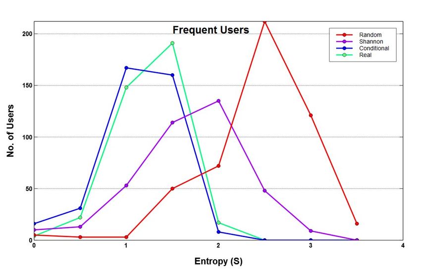
patterns across various social networks can also affect how                Random Entropy: This takes into account the number of
their check-in patterns are acquired. They, however, do not              unique locations N visited by each user i and is given as:
measure the accuracy of next-place-of-visit prediction using
distance metrics such as Euclidean distance. Moreover, the                                        SiRand = log2 (N )
types of venues at which users may check-in are not taken                where N > 0 since all users visit at least one location and
into account.                                                            also because log2 (0) is undefined.

   In [10], the authors explore human mobility predictability               Shannon Entropy: The probability of visiting every unique
by analysing a set of tweets generated by Swedish users.                 location j by each user i, summed across all locations visited
They conduct the analysis in terms of temporal history of                at least once:
mobility range showing how users disperse in space, and also

                                                                                                        N
investigate entropy and its corresponding predictability. The                              SiShan = −         pi,j log2 (pi,j )
results uncover a set of users routinely visiting some locations                                        j=1
most of the time, and occasionally exploring new places as
well. By measuring the entropy of each user’s individual                 where pi,j is the number of visits to location j by user i
trajectory, a 70% theoretical predictability is achieved. They,          divided by total visits for all locations visited by user i.
however, do not perform the actual prediction for users.
                                                                            Conditional Entropy: Checks for correlation between a
                                                                         previously visited location xt−1 and a subsequent one xt in
   In [11], the Shannon and Real predictability of a particular
                                                                         time series:
set of users are analysed and correlated with corresponding
entropy. Using Twitter data, users with at least 100 tweets are             SiCond = −                pi (xt−1 , xt ) log2 pi (xt |xt−1 )
chosen and analysis is performed based on a certain number                                xt ∈Xi xt−1 ∈Xi
of distinct locations visited by these users. The median
                                                                         where Xi is the set of all locations visited by user
value for both entropies follows a linearly increasing trend
                                                                         i, pi (xt−1 , xt ) denotes the probability of visiting the
as the number of locations increases, however, the Shannon
                                                                         ordered pair of visited locations xt−1 and xt by user i,
entropy increases at a faster rate. Similarly, the decrease in
                                                                         and pi (xt |xt−1 ) = pi (xt−1 , xt ) /pi (xt−1 ) represents the
predictability for higher number of locations is slower for
                                                                         probability of visiting the location xt at time-ordered t given
Real predictability compared to Shannon’s. Overall, this work
                                                                         a previously visited location xt−1 by user i. Only pairs that
suggests the importance of spatio-temporal correlations in
                                                                         appear in a user history are used to ensure pi (xt |xt−1 ) > 0.
visitation patterns in predicting future tweet locations. The
actual prediction for users, however, is not analysed here.
                                                                            Real Entropy: This considers the complete spatio-temporal
                                                                         information of a visit, takes into account the frequency,
   For prediction of user movements, a number of techniques
                                                                         visitation sequence and time spent.
have been used by researchers in the literature. In [12], an
                                                                                                     n         −1
                                                                                                         m=2 lm
Auto-Regressive Integrated Moving Average (ARIMA) model
is proposed to predict the spatio-temporal variations of taxi                              SiReal =
                                                                                                      n log2 (n)
passenger numbers in China. The method uses GPS traces
from 4000 taxis and achieves a prediction performance with               where lm is the length of the shortest sequence of locations
5.8% error. In [13], the authors use Mixed Markov Model                  starting at position m which does not show in the part of
(MMM) to predict pedestrian movement in Osaka, Japan                     sequences up to position m − 1.
and claim to achieve a prediction accuracy of 74.4%. Other               B. Predictability
methods such as Gradient Boosting regression tree method
                                                                            In the mobility scenario, predictability is a measure of the
(GBM) [14] and Support Vector Machine (SVM) [15] have
                                                                         future whereabouts of a user and is inversely proportional to
also been used with varying degrees of accuracy.
                                                                         entropy. The predictability Πi of user i is subject to Fano’s
                                                                         inequality [17] and can be related to the user entropy Si as:
             III. T HEORETICAL BACKGROUND
  This section presents the theoretical background about the                        Si = H(Πi ) + (1 − Πi ) log2 (Ni − 1)          (1)
concepts and methods used in this paper for data analysis.               where  H(Πi ) is the binary entropy function which is defined
                                                                         as the entropy of a Bernoulli process with the probability of
A. Entropy                                                               success Πi that can take only two values: 0 and 1.
   Entropy is a measure of the degree of randomness in a                       H(Πi ) = −Πi log2 Πi − (1 − Πi ) log2 (1 − Πi )   (2)
process. Since movement itself is a process and users usually
move between different locations, we are trying to find any               where  represents a placeholder for a particular kind of
patterns or predictable movements between the suburbs. There             entropy, and Ni is the total possible locations visited by user
are four types of entropy as mentioned in [5], [16] and [8].             i based on their history. This means that given the entropy

                                                                   436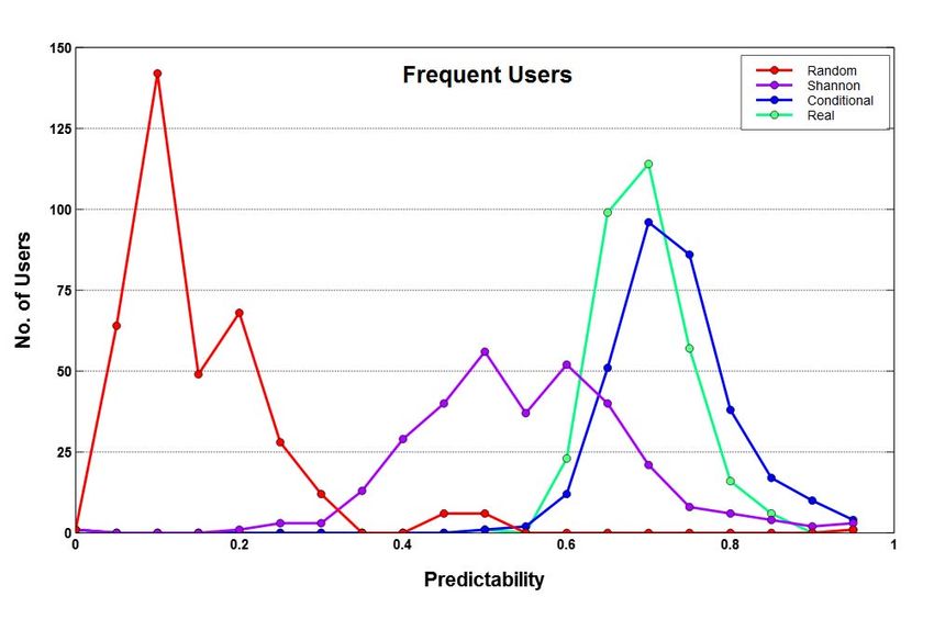
S , we can find the predictability Π by solving Equation 1
numerically. For each type of entropy, we have corresponding
type of predictability such as Random predictability, Shannon
predictability, Conditional predictability, and the Real
predictability.
It should be noted that the term “process” refers to timeline
of each user, and hence, all of the above measures are
calculated for every user in the system. Moreover, location
means the suburb where a tweet is posted, and sequence means
a time-ordered set of suburbs.
C. Markov Model
As mentioned earlier, our goal is to predict the next location Fig. 1: The number of tweets in the top 20 suburbs, and the
visited by users based upon the observation of their previous second top 20 suburbs active on Twitter in the data set.
location(s) over a period of time. The potential applications of
such analysis can include the development of location-based
services anticipating the next movement of a user or to the percentage of users making a certain minimum number
predict the spread of a disease from one place to another. of tweets throughout the data collection period. A very
This can also help in emergency situation, or understanding large share of users (79.8%) post a small number of tweets
short/long term migration patterns. For this purpose we will (between 1 and 24), while the users making a large number
use the Markov predictor. This type of predictor represents of tweets comprise of relatively much smaller percentage
the mobility behaviour of a user as a Markov model and (4.9%). This suggests that, broadly, users can be partitioned
predicts the next state based on the previous state(s). In into two groups: casual and frequent, and hence, for the
our case, the state refers to a suburb, hence, the transition analysis carried out in this paper, we separate the users who
between two states corresponds to the probability of moving have posted at least 25 tweets in the data set, and call them
from one suburb to another. The mobility behaviour is treated ‘frequent’ users, and term all other users as ‘casual’. We
as a discrete stochastic process. perform the entropy and predictability analysis for both these
groups.
IV. DATA S ET & E XPERIMENTAL S ETUP
The data set has been collected using Twitter Streaming API TABLE I: The percentage of users posting a minimum number
[18], geographically covering Australia and spanning a period of tweets in the data set. For example, 79.8% of users posted
from January 2015 till July 2016. It consists of 9462345 between 1 and 24 tweets.
tweets from 245796 unique users. For Sydney we have 947964
geo-tagged tweets and 40281 unique users, for Melbourne we No. of Tweets % of Users
Between 1 and 24 79.8
have 854821 geo-tagged tweets and 35556 unique users and Between 25 and 49 9.6
for Brisbane we have 276394 geo-tagged tweets and 14555 Between 50 and 99 5.7
unique users in the data set. For experiments, these three 100 and above 4.9
cities are chosen and only their top-20 suburbs are utilized
for the analysis. These suburbs are chosen w.r.t highest
We also do the prediction analysis for top users of each city
twitter activity since they account for the largest amount of
and discuss this in detail in §VI.
data compared to the remaining suburbs as shown in Figure 1.
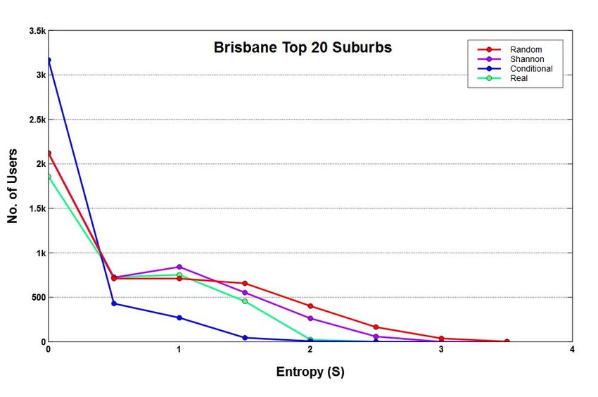
V. P RELIMINARY E NTROPY AND P REDICTABILITY
As shown in Figure 1 the top-20 suburbs of each city
capture up to four times the twitter activity than the next 20 We start with analysing the entropy and predictability of
suburbs and as we go further down, the twitter activity drops all users among top-20 suburbs of Sydney, Melbourne and
significantly. Moreover, the top-20 suburbs cover key spatial Brisbane. This is done to get an idea about how random or
areas of a city where most of the movements usually take predictable the user movements are in general. Figure 2 (a-f)
place. The movements that users make between suburbs are shows the entropy and predictability measures for the three
referred to as fluxes. cities. Since the maximum value of entropy is about 4 for
random entropy, we divide entropy range 0-4 into 8 bins with
It is also important to give consideration to the number width 0.5, and assign each user to one of these bins. For
of tweets posted by each user in the data set. The total predictability measure, we assigned users to bins with width
number of unique users posting only geo-tagged tweets in 0.05, similarly. The number of users in each bin is shown in
our data set is 105641 and Table I provides an overview of Figure 2.
437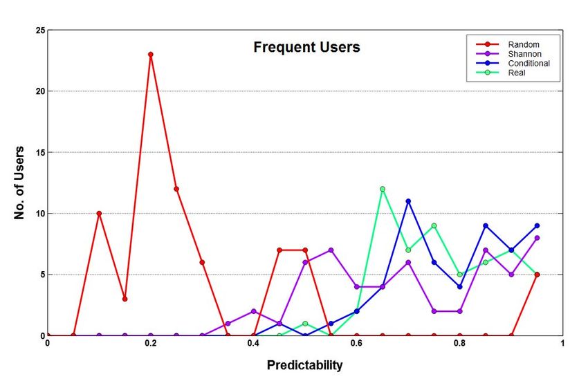
(a) (b)
(c) (d)
(e) (f)
Fig. 2: The number of users in each entropy and predictability bin in the three cities.
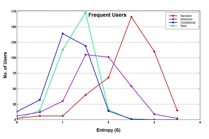
We observe that entropy distributions do not seem to follow of each other depends upon how the binning is performed for
the standard order of S Real ≤ S Cond ≤ S Shan ≤ S Rand plotting the data points.
and the corresponding predictability distributions also exhibit
coarse trend. This suggests that twitter users have wide ranging A. Frequent vs Casual User Groups
behaviour reflecting some degree of randomness as well as We compute various entropies and predictabilities for fre-
some regularity. If users with similar mobility behaviour, either quent and casual users belonging to Sydney as shown in
with high randomness or high regularity are separated into Figure 3.
different groups, then it is possible that highly predictable We can see that the behaviour of frequent users is different
users may be identified more easily. Visually, the extent to from casual users whereas the casual users still show coarse
which entropy and predictability measures are mirror image distributions like the case of all users as shown in Figure
438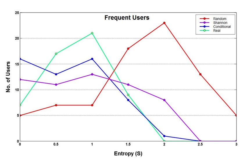
(a)                                                            (b)

                                     (c)                                                            (d)
                                              Fig. 3: Sydney’s frequent vs. casual users

2 (a, b). Table II summarises the percentages, averages and              than 50% of overall movements between its suburbs.
upper bound threshold for each group of all three cities’ users.
                                                                            The entropy measure can also be used to infer the
                                                                         significance of Markov chain transition probabilities i.e.
          TABLE II: User behaviour for each city
                                                                         whether the next location is highly predictable based on
          Users     No. of Fluxes per User   % of     % of
                                                                         current location. On the other hand, predictability measure
                                             Users    Fluxes             can be perceived as a theoretical upper bound of prediction
                    Max     Avg     StDev                                that can possibly be achieved using a suitable prediction
   Syd   Frequent    198     46.5    27.9    3.06%    29.17%             algorithm. In Figure 4, we show the plots for remaining two
          Casual      24     3.57     4      96.94%   70.83%
   Mel   Frequent   1218    48.43   69.67    3.00%    29.67%             cities.
          Casual      24     3.56    3.98    97.00%   70.33%
   Bri   Frequent   6044     160    809.4    2.08%    53.72%
          Casual      24     2.94    3.39    97.92%   46.28%
                                                                            In Figure 4 (c, g), we see that entropies of casual users
                                                                         do not follow the standard ordering rule and such users are
                                                                         difficult to analyse. The large proportion of very low entropy
   It is expected that frequent users will have different                values corresponds to a large number of users having a small
prediction characteristics than casual users and we analyse              number of fluxes, and prediction accuracy for these users is
the most predictable users in section VI. We also observe                unlikely to be high [19]. In contrast, the entropy distributions
that average value for frequent users is much higher than                of frequent users look better, exhibiting normal distribution as
that of casual users, and although the percentage of number              shown in Figure 4 (a, e). This also suggests that in general,
of frequent users is much smaller than the casual users,                 we have reasonably differentiated and grouped the users
the frequent users still account for a proportionately good              together from entropy point of view. It is important to note
percentage of overall movements. Brisbane shows a different              that estimation of various types of entropies and their standard
trend whereby its average value is more than three times that            order becomes exact only for infinitely long sequences where
of Sydney and Melbourne and its frequent users record more               all locations and transition probabilities between them can

                                                                   439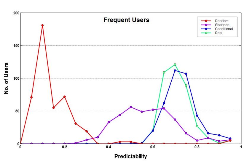
(a) Melb. frequent entropy                             (b) Melb. frequent predictability

(c) Melb. casual entropy                                (d) Melb. casual predictability

(e) Bris. frequent entropy                              (f) Bris. frequent predictability

 (g) Bris. casual entropy                                (h) Bris. casual predictability
            Fig. 4: Frequent vs Casual users entropy and predictability

                                        440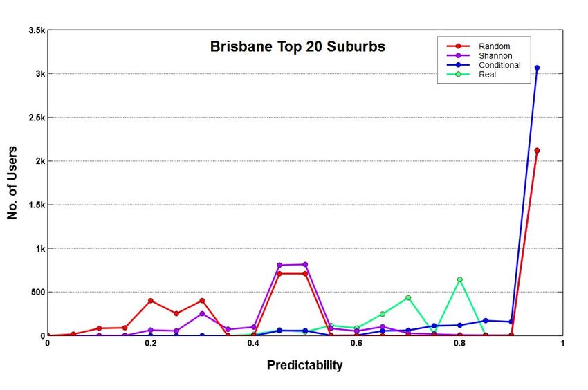
accurately be calculated [19].                                                      TABLE IV: Average predictability for cities

   Table III shows the average values for all types of entropies                    City                  Avg. Predictability
                                                                                              Random     Shannon     Conditional   Real
for all three cities and we utilise these figures to get further                   Sydney       0.17        0.59          0.75      0.73
insights.                                                                        Melbourne     0.16        0.57          0.75      0.71
                                                                                 Brisbane      0.32        0.73          0.82      0.79

TABLE III: Average entropies for cities and their user groups

   City/User Group     RandEnt   ShanEnt    CondEnt    RealEnt             history of locations. This means prediction problem can be
   Sydney/Frequent       2.7       1.95       1.4       1.49               presented where the actual predictability can be represented
  Melbourne/Frequent     2.71      2.01       1.4       1.54               by the conditional predictability whereby considering just
  Brisbane/Frequent      1.9       1.16       0.92      1.06               the last location returns almost the same predictability as if
                                                                           considering the entire previous history of movements.
   For Sydney frequent users, the averages for random,
                                                                              In literature, studies have been conducted about predictabil-
Shannon, conditional and real entropies are 2.7, 1.95, 1.4
                                                                           ity analysis using mobile phones. Song et al. [5], Lu et al. [6]
and 1.49 respectively. It means that the next location for a
                                                                           and Qin et al. [7] found 93%, 88% and 78% predictability for
user could randomly be out of possible 2rand ≈ 22.7 ≈ 7
                                                                           users respectively. Here, the predictability for Brisbane users
locations where each location is unique one. If we count the
                                                                           is close to the calculation of Qin et al. [7]. However, both Song
movement frequency, then this uncertainty will be shown
                                                                           et al. [5] and Qin et al. [7] did not further pursue their work to
by Shannon entropy, hence, 2Shan ≈ 21.95 ≈ 4 locations.
                                                                           do actual prediction to show whether their high predictability
So Shannon entropy suggests fewer highly probable next
                                                                           results can be achieved in practice. On the other hand, Lu
locations than random entropy. If we take into account the
                                                                           et al. [6] used a Markov Chain model to perform prediction
sequence of locations visited, then the conditional entropy
                                                                           and achieved an accuracy at par with their predictability level
will be 2cond ≈ 21.4 ≈ 3 locations. Finally, considering the
                                                                           using the first order Markov model. In the following section,
whole history of movements, the real entropy average of 1.49
                                                                           we explore the prediction problem to get further insights into
also yields 21.49 ≈ 3 locations. For Melbourne, the number
                                                                           the movement patterns of Twitter users.
of possible locations based on each type of entropy are
7(random), 4(Shannon), 3(conditional) and 3(real) whereas                             VI. P REDICTION OF N EXT L OCATION
for Brisbane these numbers are 4(random), 2(Shannon),
                                                                              Prediction estimates the next location based on the transition
2(conditional) and 2(real).
                                                                           probability matrix. Given a current location, the next location
                                                                           with the highest probability from the transition matrix
   It is observed that real entropy is close to conditional                assembled from the training set is used as the estimated next
entropy, suggesting the fact that entropy is strongly determined           location. We take the entire data set for users and investigate
by location history with most of the information in last visited           the previous location for a record to determine the chance of
location.                                                                  correctly predicting the next location. Specifically, we choose
                                                                           the top most predictable users for each city as per their
   Next we look at predictability as shown in Figure 4                     theoretical real predictability values and do the prediction for
(b,d,f,h). Examining the frequent users, we find that average               them to see what their prediction accuracy is like. We use the
real predictability, ΠReal , for Sydney is 0.73, for Melbourne             first order Markov Chain predictor to conduct this analysis.
it is 0.71, whereas for Brisbane it is 0.79. The predictability            For each user, the origin-destination (OD) transition matrix
values suggest there is a possibility that about 73% of                    and their probabilities are calculated based on one previous
Sydney, 71% of Melbourne and 79% of Brisbane users’                        state. For all the days that a user is active in the whole data
whereabouts can possibly be predicted with the help of a                   set, we use the first 80% of the days as training period, and
good prediction algorithm, whereas the remaining 27%, 29%                  the last 20% as the test period. The predictor checks in which
and 21% users of these cities are difficult to predict. Hence,              suburbs the users have been mostly active in the training set
the predictability measure provides a theoretical upper bound              and calculates prediction for the corresponding suburbs in the
of the prediction algorithm performance [19]. In other words,              test set. The accuracy measure is calculated as the number of
for actual prediction accuracy, this is the target that could              correct predictions divided by the total number of predictions
possibly be achieved by a good algorithm [6]. Table IV shows               (correct plus incorrect).
the average predictability values for these cities.
                                                                             After doing our prediction analysis for the top predictable
   It can be seen that real predictability is close to conditional         users of each city, we report the findings in Table V.
predictability and this clearly suggests that most of the                    It shows the prediction accuracies for top 1%, 5% and 10%
information about the probable next location is held in the                of users (in terms of mobility) for each city along with their
current location, implying a weak dependence on the previous               corresponding theoretical predictability ranges. Among all

                                                                     441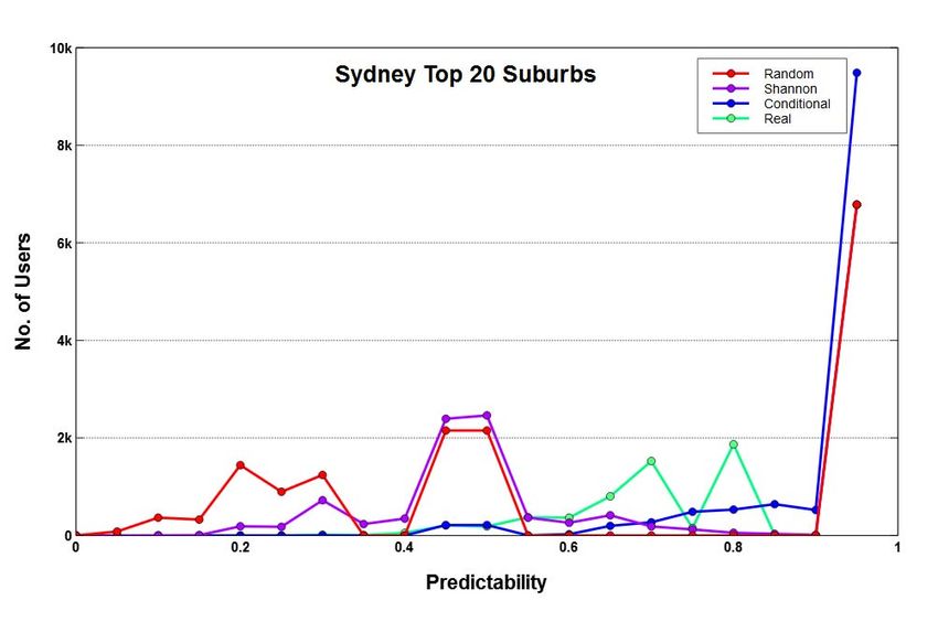
TABLE V: Prediction accuracy & Real predictability                   Future work can involve tracking the movements of frequent
                                                                         users itself over a period of time with a broader goal to
    City      Top 1%   Users    Top 5%   Users    Top 10% Users          detect change in their routine activity patterns and exploit that
              Accu.    Pred.    Accu.    Pred.    Accu.   Pred.
                                                                         information for some useful purpose.
  Brisbane    100%     All 1    100%     All 1    76.6%  0.94-1
  Melbourne   63.3%    0.88-1   47.1%    0.81-1   49.2%  0.79-1                                        R EFERENCES
   Sydney     100%     All 1     53%     0.83-1   54.8%  0.80-1
                                                                          [1] X. Song, Q. Zhang, Y. Sekimoto, R. Shibasaki, N. J. Yuan, and
                                                                              X. Xie, “Prediction and simulation of human mobility following natural
                                                                              disasters,” ACM Transactions on Intelligent Systems and Technology,
                                                                              vol. 8, no. 2, pp. 29:1–29:23, Nov. 2016.
cities, Brisbane users record highest prediction accuracy and             [2] X. Song, H. Kanasugi, and R. Shibasaki, “Deeptransport: Prediction and
can be best related to their theoretical predictability values.               simulation of human mobility and transportation mode at a citywide
Up to first 5% of its users can completely be predicted and                    level,” in 25th International Joint Conference on Artificial Intelligence,
                                                                              ser. IJCAI’16. AAAI Press, 2016, pp. 2618–2624.
after that the prediction accuracy decreases. In general, we can          [3] Q. Wang and J. E. Taylor, “Process map for urban-human mobility
say that the results correspond with theoretical calculations                 and civil infrastructure data collection using geosocial networking plat-
for average real predictability in Table IV which is highest                  forms,” Journal of Computing in Civil Engineering, vol. 30, no. 2, p.
                                                                              04015004, 2016.
for Brisbane than the rest of the cities.                                 [4] S. F. Khan, N. Bergmann, R. Jurdak, B. Kusy, and M. Cameron,
                                                                              “Mobility in cities: Comparative analysis of mobility models using geo-
   For Melbourne, we observe lower prediction accuracy than                   tagged tweets in australia,” in 2017 IEEE 2nd International Conference
                                                                              on Big Data Analysis (ICBDA) Beijing, pp. 816–822.
Brisbane. The maximum accuracy that we could achieve here                 [5] C. Song, Z. Qu, N. Blumm, and A.-L. Barabási, “Limits of predictability
is 63.3% and this is for top 1% of users only. Subsequent                     in human mobility,” Science, vol. 327, no. 5968, pp. 1018–1021, 2010.
sets of users have even lower accuracy and we infer that                  [6] X. Lu, E. Wetter, N. Bharti, A. J. Tatem, and L. Bengtsson, “Approaching
                                                                              the limit of predictability in human mobility,” Scientific reports, vol. 3,
users in Melbourne are not as predictable as those in Brisbane.               p. 2923, 2013.
                                                                          [7] S.-M. Qin, H. Verkasalo, M. Mohtaschemi, T. Hartonen, and M. Alava,
   For Sydney, we note that top 1% of users have 100%                         “Patterns, entropy, and predictability of human mobility and life,” PLOS
                                                                              One, vol. 7, no. 12, p. e51353, 2012.
accuracy but the top 5% users have accuracy dropping down                 [8] R. Sinatra and M. Szell, “Entropy and the predictability of online life,”
to 53%. This suggests that except for a few users, most of the                Entropy, vol. 16, no. 1, pp. 543–556, 2014.
users have comparatively larger variation in their movements.             [9] D. Teixeira, M. Alvim, and J. Almeida, “On the predictability of a
                                                                              user’s next check-in using data from different social networks,” in
Overall, this points to a possible different style of movements               Proceedings of the 2nd ACM SIGSPATIAL Workshop on Prediction of
in these two cities and users in general are harder to predict                Human Mobility, ser. PredictGIS 2018, New York, NY, USA, 2019, pp.
for their next movements.                                                     8–14.
                                                                         [10] Y. Liao and S. Yeh, “Predictability in human mobility based on
                                                                              geographical-boundary-free and long-time social media data,” in 21st
   The prediction for users based on their movement patterns                  International Conference on Intelligent Transportation Systems (ITSC),
can help identify the differences between them, and the com-                  Nov 2018, pp. 2068–2073.
                                                                         [11] R. Jurdak, K. Zhao, J. Liu, M. AbouJaoude, M. Cameron, and D. Newth,
parison of various cities can also reveal the mobility dynamics               “Understanding human mobility from Twitter,” PLOS One, vol. 10, no. 7,
in a broader perspective. Despite using an identical criteria                 p. e0131469, 2015.
for choosing users, we observed heterogeneity among cities               [12] X. Li, G. Pan, Z. Wu, G. Qi, S. Li, D. Zhang, W. Zhang, and Z. Wang,
                                                                              “Prediction of urban human mobility using large-scale taxi traces and its
in terms of predicting the next location of its users.                        applications,” Frontiers of Computer Science, vol. 6, no. 1, pp. 111–121,
                                                                              2012.
                     VII. C ONCLUSIONS                                   [13] A. Asahara, K. Maruyama, A. Sato, and K. Seto, “Pedestrian-movement
   This work explored the movement patterns of Twitter users                  prediction based on mixed Markov-chain model,” in 19th ACM SIGSPA-
                                                                              TIAL international conference on advances in geographic information
in three Australian cities and it is observed that users can                  systems, 2011, pp. 25–33.
generally be split into two groups: frequent and casual based            [14] Y. Zhang and A. Haghani, “A gradient boosting method to improve
on their activity characteristics. The randomness and regularity              travel time prediction,” Transportation Research Part C: Emerging
                                                                              Technologies, vol. 58, pp. 308–324, 2015.
of these user groups are investigated using the concepts of              [15] A. Lopez Aguirre, I. Semanjski, and S. Gautama, “Forecasting travel
entropy and predictability. Brisbane users have highest average               behaviour from crowdsourced data with machine learning based model,”
Real predictability of 79% compared to other cities. In terms                 in Fifth International Conference on Data Analytics, vol. 5.          The
                                                                              International Academy, Research and Industry Association, 2016, pp.
of actual prediction too, the top users in Brisbane have higher               93–99.
prediction accuracy of 100% for top 5% users, and 76.6%                  [16] R. Gallotti, A. Bazzani, M. Degli Esposti, and S. Rambaldi, “Entropic
for top 10% users. In comparison, the Sydney and Melbourne                    measures of individual mobility patterns,” Journal of Statistical Mechan-
                                                                              ics: Theory and Experiment, vol. 2013, no. 10, p. P10022, 2013.
users have much lower prediction accuracy, and overall, this             [17] T. M. Cover and J. A. Thomas, Elements of information theory. John
suggests heterogeneity among the cities. The ability to predict               Wiley & Sons, 2012.
the next location of users can have applications such as antic-          [18] Twitter.           (2015,          Jun.)         Streaming          APIs.
                                                                              https://dev.twitter.com/streaming/overview.
ipating the use and management of resources being offered                [19] I. B. I. Purnama, N. Bergmann, R. Jurdak, and K. Zhao, “Characterising
at a certain place. It is therefore important to identify the                 and predicting urban mobility dynamics by mining bike sharing system
movements which are most predictable and such movements                       data,” in IEEE 12th International Conference on Ubiquitous Intelligence
                                                                              and Computing (UIC), 2015, pp. 159–167.
in turn are expected from frequent users. These users can
be apprised of any update about their probable next location.

                                                                   442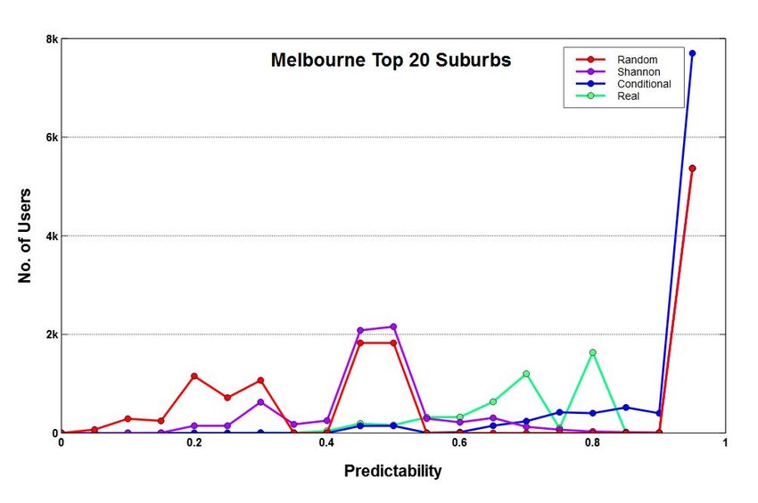
You can also read