Virtual Quake: Statistics, Co-Seismic Deformations and Gravity Changes for Driven Earthquake Fault Systems
←
→
Page content transcription
If your browser does not render page correctly, please read the page content below
International Association of Geodesy Symposia manuscript No.
(will be inserted by the editor)

Virtual Quake: Statistics, Co-Seismic Deformations and
Gravity Changes for Driven Earthquake Fault Systems
Kasey W. Schultz · Michael K. Sachs · Eric M. Heien · Mark R. Yoder ·
John B. Rundle · Don L. Turcotte · Andrea Donnellan

Received: xxxxx, 2014 / Accepted: xxxxx, 2015

Abstract With the ever increasing number of geode-              1 Introduction
tic monitoring satellites, it is vital to have a variety
of geophysical simulations produce synthetic datasets.          The purpose of this paper is to introduce a subset of the
Furthermore, just as hurricane forecasts are derived            wide range of applications of the Virtual Quake (VQ)
from the consensus among multiple atmospheric mod-              earthquake simulator, originally developed by Rundle
els, earthquake forecasts cannot be derived from a single       [1988a,b]. Virtual Quake makes several simplifications
comprehensive model. Here we present the functionality          about the earth that should be highlighted. VQ simu-
of Virtual Quake (formerly known as Virtual Califor-            lates fault interactions a single layer elastic half-space
nia), a numerical simulator that can generate sample            with no viscoelasticity. Furthermore, unlike physical fault
co-seismic deformations, gravity changes, and InSAR             systems where fault geometry is dynamic over geologic
interferograms in addition to producing probabilities           time periods, VQ makes a simplification by assuming
for earthquake scenarios.                                       a geometrically static fault system by using backslip
    Virtual Quake is now hosted by the Computational            to build stress [Rundle et al., 2006c]. This simplifica-
Infrastructure for Geodynamics. It is available for down-       tion reflects the goal of Virtual Quake simulations, to
load and comes with a user manual. The manual in-               explore seismicity in today’s fault systems rather than
cludes a description of the simulator physics, instruc-         modeling their long term evolution or the short term
tions for generating fault models from scratch, and a           dynamics. For detailed descriptions of the Virtual Quake
guide to deploying the simulator in a parallel comput-          simulator see Sachs et al. [2012], Heien and Sachs [2012].
ing environment. Virtual Quake is continuously refined              Even though the current version of Virtual Quake
and updated, and we are currently preparing a suite of          does not account for the layered three dimensional Earth,
visualization and analysis tools in an upcoming release.        Tullis et al. [2012a] confirmed that the current VQ simu-
http://geodynamics.org/cig/software/vq/                         lations are consistent with both the observed seismicity
                                                                in California and with independent California fault sys-
Keywords GENAH · Virtual California · Virtual                   tem simulations. Yikilmaz et al. [2010] showed that Vir-
Quake · earthquake forecasting                                  tual Quake simulations of the Nankai Trough in Japan
                                                                are consistent with observed earthquake sequences.
                                                                    Following Hayes et al. [2006] we have added a more
Kasey W. Schultz · Michael K. Sachs · Mark R. Yoder · John      generalized method for modeling co-seismic gravity changes
B. Rundle
Department of Physics, University of California-Davis, One
                                                                for simulated earthquakes on arbitrary faults with Vir-
Shields Ave. Davis, CA 95616                                    tual Quake [Schultz et al., 2014]. We utilize a custom
E-mail: kwschultz@ucdavis.edu                                   version of the gravity Green’s functions presented in
John B. Rundle · Don L. Turcotte · Eric M. Heien                Okubo [1992] for faulting in an elastic half-space. Though
Department of Earth and Planetary Sciences, University of       VQ does not yet support a three dimensional layered
California-Davis                                                earth, these gravity Green’s functions have been ex-
Andrea Donnellan                                                tended for a dislocations in a three dimensional earth
Jet Propulsion Laboratory, California Institute of Technology   and are presented in Sun et al. [2009]. These equations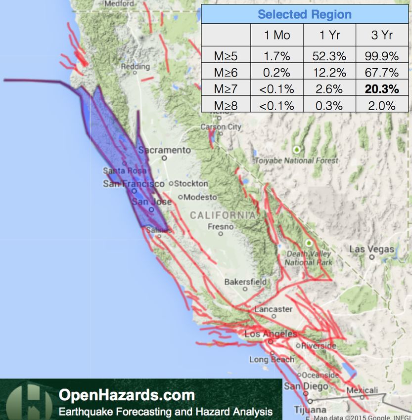
2                                                                                                Kasey W. Schultz et al.

have shown good agreement with observed co-seismic        the properties of modern earthquake simulators and a
gravity signals observed by the GRACE satellite for the   comparison of Virtual California to other simulators see
2011 Tohoku-Oki earthquake [Matsuo and Heki, 2011]        Tullis et al. [2012b]. For a comparison of Virtual Califor-
and for the 2010 Central Chile earthquake [Heki and       nia simulations to those of other earthquake simulators
Matsuo, 2010].                                            using the same fault model see Tullis et al. [2012a].
    Over the past decade, Virtual Quake has been part
of a multi-disciplinary effort to better understand, pre- 3 Surface Patterns
dict, and respond to earthquake hazards known as QuakeSim
[Donnellan et al., 2006]. The QuakeSim team aims to       Virtual Quake calculates co-seimic deformations, In-
develop a solid Earth science framework for modeling      SAR (Synthetic Aperture Radar Interferometry) pat-
and understanding earthquake and tectonic processes.      terns, co-seismic gravity changes and more for arbitrar-
As part of the QuakeSim team, Virtual Quake was se-       ily complex fault geometries [Rundle et al., 2006c, Sachs
lected as a co-winner of NASA’s 2012 Software of the      et al., 2012, Schultz et al., 2014]. VQ calculates these
Year award [NASA, 2012].                                  surface patterns by using fault geometry and co-seismic
                                                          slips as input to a specific set of Green’s functions. Since
2 Virtual Quake Simulator                                 Virtual Quake partitions the fault system into finite
                                                          boundary elements embedded in an elastic half-space,
Virtual Quake (VQ) is a boundary element code that        the Green’s functions are a logical extension of the sim-
simulates realistically driven fault systems based on     ulator’s capability. For surface deformation and InSAR
stress interactions. VQ is designed to explore the long   calculations we use the Green’s functions presented in
term statistical behavior of topologically complex fault  Okada [1992], and for gravity and potential changes we
networks [Rundle, 1988a,b, Rundle et al., 2006a,b,c].     use the Green’s functions presented in Okubo [1992].
The most recent version of VQ is a modern scientific          These surface patterns reveal changes in the dy-
code that simulates earthquakes in a high performance     namic   variables associated with the earthquake cycle
computing environment [Sachs et al., 2012, Heien and      that  are  inherently unobservable like the stress field.
Sachs, 2012]. VQ simulates many thousands of years of     Rundle et al. [2000] developed a technique for describ-
seismic history on fault networks with any physically     ing the evolution of space-time patterns as a “pattern
realizable geometry.                                      dynamics”. Tiampo et al. [2002] applied this analysis
    VQ consists of three major components: a fault model, on seismicity data in southern California and argued for
simulation physics, and an event model. The fault model   the development of more sophisticated computer sim-
is the simulation input and it can be changed to any ar-  ulations to carry out a more systematic analysis. Our
bitrary fault geometry and function properly the simu-    goal is to provide a tool for generating physics-based
lation physics and event model. The simulation physics    catalogs of modeled geophysical fields arising only from
is based on fault stress via the accumulation of a slip   fault-fault interactions across entire fault networks. In
deficit — the amount of slip each fault should move in a  the future, these catalogs may help reveal characteristic
given time period given the long term slip rate. Actual   patterns associated with high seismic risk or serve the
values of stress are computed by a set of quasi-static    data pipeline of satellite-based monitoring systems.
elastic interactions given in Rundle et al. [2006a].
    VQ initiates simulated earthquakes using both static      3.1 Gravity Green’s Functions
and dynamic friction laws. Slip during a simulated earth-
quake is triggered by the stress on a fault element reach-    The solutions presented by Okubo [1992] allow calcula-
ing the failure threshold as specified in the fault model,    tion of gravity changes for dislocations on finite faults
this is static failure. Elements on the same fault are also   in an elastic half-space. Following Hayes et al. [2006] we
allowed to slip — even if they have not reached failure       have implemented a custom version of these equations
stress — if the stress is at least 50% of the threshold       in Virtual Quake that allow modeling of gravity changes
value. This dynamic failure condition can be tuned and        for arbitrary fault geometry and slip. For a detailed ex-
is used to control rupture propagation for simulated          planation of the Virtual Quake implementation of the
earthquakes.                                                  Okubo’s equations see Schultz et al. [2014].
    Hereafter Virtual Quake simulations of the Califor-           Figure 1 shows the co-seismic gravity pattern pro-
nia fault system are referred to as Virtual California        duced by Virtual California for a M=7.69 simulated
(VC). For example, if we simulated the Japan fault sys-       earthquake rupturing the northern San Andreas Fault.
tem then we would refer to that application of Virtual        This is a model of the total gravity signal at the sur-
Quake as Virtual Japan. For a detailed explanation of         face including contribution from surface displacement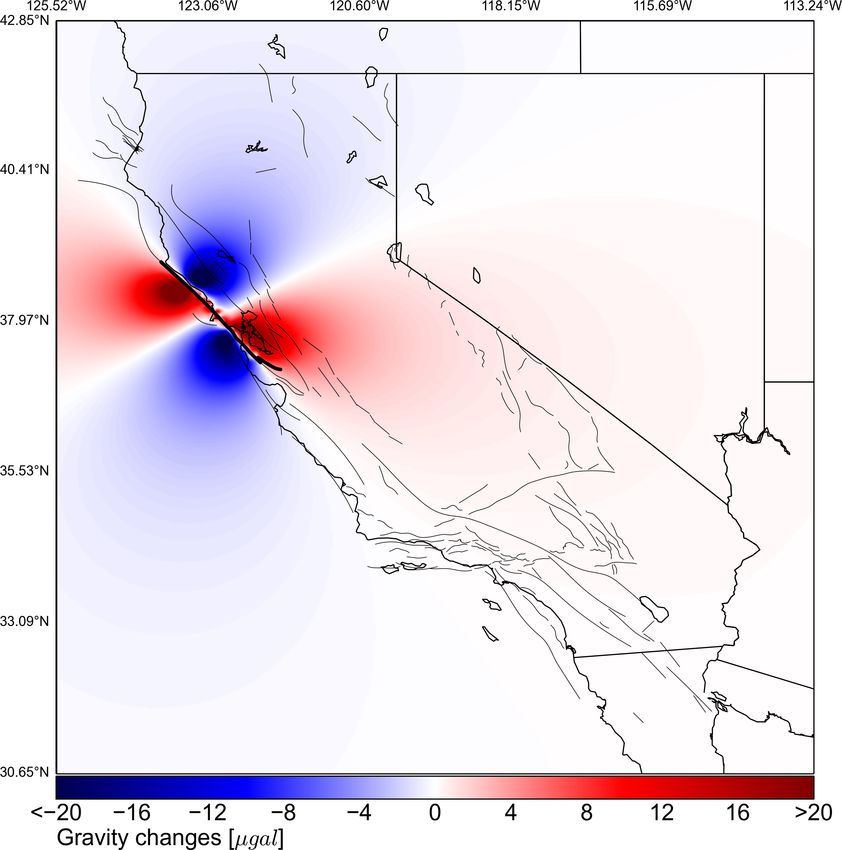
Virtual Quake                                                                                                               3

Fig. 1 Gravity Green’s function solutions for co-seismic slips   Fig. 2   Simulated InSAR interferogram for co-seismic slips
from a magnitude 7.69 VC simulated earthquake on the San         from a magnitude 7.69 VC simulated earthquake on the San
Andreas Fault. The color unit is microGals (10−8 m/s2 ), fault   Andreas Fault. View angles: azimuth = 30◦ , elevation = 40◦ ,
rupture is shown in dark black.                                  fault rupture is shown with bold white lines.

and from compression and dilatation. The dark black              a detailed comparison of observed northern California
line indicates the fault sections that slipped during the        seismicity and simulated seismicity by adding background
simulated event. Our model is a single layer elastic half-       seismicity to an early Virtual California simulation.
space model and it does not account for viscoelasticity,             Here we derive the probabilities for a northern Cal-
elastic discontinuities, or the three dimensional layered        ifornia earthquake scenario using a recent 50,000 year
earth.                                                           Virtual California simulation of the allcal2 California
                                                                 fault system model. The fault model, which is parti-
                                                                 tioned into more than 14,000 3km×3km square bound-
3.2 Displacement Green’s Functions and InSAR
                                                                 ary elements, is described in detail in Tullis et al. [2012b].
Virtual Quake employs a custom version of the dis-               We follow Rundle et al. [2005] and illustrate our ap-
placement Green’s functions given in Okada [1992] to             proach using the Virtual California simulation to ob-
produce simulated co-seismic deformation maps and In-            tain recurrence statistics and construct the probability
SAR interferograms. Using simulated co-seismic slip dis-         distributions. We then compare earthquake probabili-
tributions and the Okada Green’s functions, Virtual              ties generated by Virtual California to an independent
Quake can generate entire catalogues of InSAR inter-             forecasting method.
ferograms and surface deformation maps for arbitrary
observing angles. Figure 2 shows the modeled InSAR               4.1 Weibull distribution
interferogram for the same M = 7.69 simulated earth-
                                                                 A probability distribution that is used frequently for
quake shown in Figure 1, as seen by observing with an
                                                                 earthquake recurrence statistics is the Weibull distri-
azimuthal angle of 30◦ and elevation angle of 40◦ .
                                                                 bution [Rundle et al., 2005]. Yakovlev et al. [2006] and
                                                                 Abaimov et al. [2008] showed that the Weibull distribu-
4 Virtual California Forecasts                                   tion fit early Virtual California simulations of the San
                                                                 Andreas Fault. The Weibull distribution specifies the
Van Aalsburg et al. [2007] and Van Aalsburg et al.               fraction of recurrence times P (t) that are less than t,
[2010] first studied the feasibility of computing earth-         and is expressed as
quake probabilities with an early version of Virtual Cal-
ifornia and compared the forecasting method with fore-                          "   #
                                                                                     β
casts produced by the Working Group on California                                  t
                                                                 P (t) = 1 − exp −      ,                                 (1)
Earthquake Probabilities. Yikimaz et al. [2011] made                               τ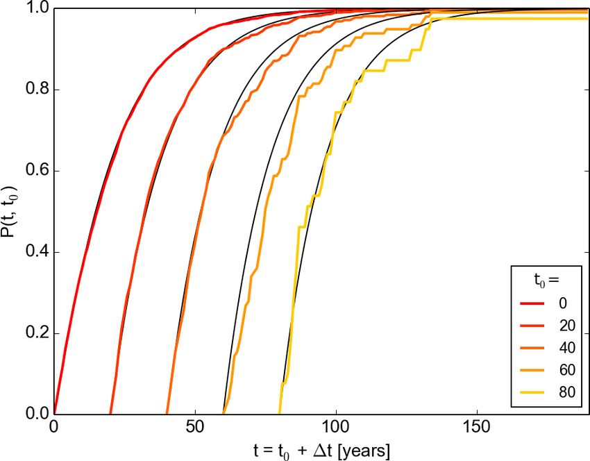
4 Kasey W. Schultz et al.
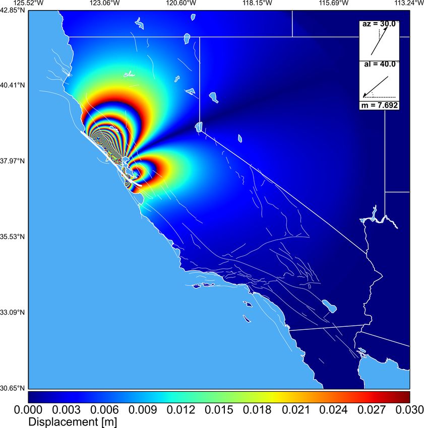
Fig. 4 Conditional cumulative probability P (t, t0 ) of a mag-
nitude ≥ 7.0 earthquake on the forecasted faults (figure 3).
The distribution is evaluated at t = t0 + ∆t, with the last
Fig. 3 Virtual California fault sections targeted for the
earthquake occurring t0 years ago, computed for various t0 .
northern California forecast, including the northern San An- The red line shows the Weibull distribution fit to the data
dreas fault. with β = 1.089 and τ = 20.92 years.
where β and τ are fitting parameters [Sieh et al.,
1989, Sornette and Knopoff, 1997]. The Weibull dis- The cumulative conditional probability of an M ≥ 7.0
tribution is also extended to a cumulative conditional earthquake occurring on the forecasted faults P (t, t0 )
distribution at a time t given that the last M ≥ 7.0 earthquake on
these faults occurred t0 years ago is plotted in Figure 4
" for multiple values of t0 . The conditional Weibull distri-
β β #
t0 t bution (2) is fit to the simulation-derived distribution
P (t, t0 ) = 1 − exp − . (2)
τ τ and is shown as the smooth black curves in Figure 4,
with β = 1.089 and τ = 20.92 years.
Equation 2 defines the cumulative conditional prob- In addition to the distribution of recurrence times,
ability that an earthquake will have occurred at time t we compute the distribution of waiting times ∆t until
after the last earthquake given that the last earthquake the next large earthquake. The waiting time ∆t is mea-
occurred a time t0 years ago. sured forward from the present, such that t = t0 + ∆t.
We express our results in terms of the conditional cu-
4.2 Northern California Forecast M ≥ 7.0 mulative probability P (t, t0 ) that an earthquake will
occur in the waiting time ∆t = t − t0 , given that the
The Virtual California simulation data that are funda- last major earthquake occurred t0 years ago, these dis-
mental in generating earthquake probabilities are the tributions are shown in Figure 5 for waiting times with
recurrence times, defined as the time between successive 25%, 50%, and 75% probability.
large earthquakes. Following the methods outlined in If we define the last observed earthquake with M ≥
Rundle et al. [2005], we compute the cumulative prob- 7.0 in northern California to be the magnitude 7.0 Loma
ability distributions and waiting times until the next Prieta earthquake in 1989, then that determines t0 =
earthquake on a selected subset of faults directly from 2015 − 1989 = 26 years, shown as the vertical dashed
a set of simulated recurrence times. line in Figure 5. The relatively constant waiting times
We consider earthquakes on the major faults in north- as a function of t0 combined with the fitted Weibull
ern California, including the northern San Andreas and parameter β = 1.089 being nearly 1 implies that the
surrounding faults, shown in Figure 3. Over the 50,000 M ≥ 7.0 earthquakes on faults shown in Figure 3 are
year simulation there are 2463 earthquakes with mo- occurring randomly. A Weibull distribution with β ∼ 1
ment magnitudes M ≥ 7.0 that cause slip on at least behaves like a Poisson process with the time to the
one of these faults. These earthquakes have an average next event independent of previous events [Sornette and
recurrence time of 20.2 years, with a maximum of 190.4 Knopoff, 1997]. This behavior is expected as the subset
years. From these data we construct the distribution of of faults is weakly correlated and contains multiple ma-
recurrence times t, defined as the time between succes- jor faults capable of M ≥ 7.0 earthquakes, each with
sive earthquakes on the selected faults with M ≥ 7.0. its own recurrence interval.Virtual Quake 5
Fig. 5 The waiting times for the next magnitude ≥ 7.0 earth-
quake on the northern California faults, as a function of time
since the last earthquake, t0 . The dark line indicates the me-
dian waiting time (50% probability), and the upper and lower
edges of the yellow band represent the waiting times with 75%
and 25% probability respectively. The vertical dashed line de- Fig. 6 The Northern California forecast as computed by
notes t0 = 26 years, the time elapsed since the M=7.0 Loma OpenHazards (openhazards.com/viewer) for the region se-
Prieta earthquake in 1989. lected in blue. This forecast states there is a 20.3% chance
of a M ≥ 7.0 earthquake within 3 years, compared to the VC
computed probability of 14.2%.The UCERF2 fault model is
in red.
4.3 Comparing to Independent Method
5 Conclusions and Discussion
We have selected to use the earthquake forecasting web- Here we have introduced and highlighted a few applica-
site OpenHazards.com to compute earthquake proba- tions of Virtual Quake. We have illustrated how Virtual
bilities and compare with our Virtual California fore- Quake can be used to generate catalogs of thousands of
cast. The website computes the probabilities of earth- maps of geophysical observables like co-seismic gravity
quakes of various magnitudes within a selected region changes and InSAR interferograms. We have also shown
by employing the natural time Weibull method (NTW). that Virtual Quake can produce earthquake probabili-
This model uses small earthquakes to forecast the oc- ties that are fairly consistent with a more sophisticated
currence of large earthquakes. The basic idea of their time-dependent forecasting method.
method is to compute large earthquake probabilities Virtual Quake is now hosted by the Computational
using the number of small earthquakes (updated daily Infrastructure for Geodynamics (CIG). It is available
from the ANSS catalog) that have occurred in a region for download and comes with a user’s manual that de-
since the last large earthquake. This forecasting method scribes simulator physics in detail, how to create fault
is described in detail in Rundle et al. [2012] and Holli- models, and how to run the simulator in a variety of
day et al. [2014]. computing environments.
http://geodynamics.org/cig/software/vq/
Figure 6 shows the Northern California region se-
lected for comparison to the Virtual California fore- Acknowledgements This research was supported by National
cast, with the same fault model used in the VC simula- Aeronautics and Space Administration (NASA) Earth and
Space Science fellowship number NNX11AL92H. The release
tion shown in red. The forecast generated from their version of Virtual California and the Users’ Manual are hosted
Hazards Viewer — www.openhazards.com/viewer — by the Computational Infrastructure for Geodynamics which
is completely independent from the physics governing is supported by NSF Grant EAR-0949446.
the Virtual California simulator and completely inde-
pendent from how VC computes probabilities. Taking
the VC conditional probabilities from Figure 4, we find References
there is a 14.2% chance of a M ≥ 7.0 earthquake oc-
S. Abaimov, D. Turcotte, R. Shcherbakov, J. Rundle,
curring on the faults shown in Figure 3 in the next 3
G. Yakovlev, C. Goltz, and W. Newman. Earthquakes:
years. OpenHazards computes a 20.3% probability for Recurrence and interoccurrence times. Pure and Applied
a M ≥ 7.0 earthquake occurring anywhere within the Geophysics, 165(3-4):777–795, 2008.
blue region shown in Figure 6 within the next 3 years.6 Kasey W. Schultz et al.
A. Donnellan, J. Rundle, G. Fox, D. McLeod, L. Grant, M. K. Sachs, E. M. Heien, D. L. Turcotte, M. B. Yikilmaz,
T. Tullis, M. Pierce, J. Parker, G. Lyzenga, R. Granat, J. B. Rundle, and L. Kellogg. Virtual California Earth-
and M. Glasscoe. Quakesim and the solid earth research quake Simulator. Seismological Research Letters, 83(6):973–
virtual observatory. Pure and Applied Geophysics, 163(11- 978, 2012.
12):2263–2279, 2006. K. Schultz, M. Sachs, E. Heien, J. Rundle, D. Turcotte, and
T. J. Hayes, K. F. Tiampo, J. B. Rundle, and J. Fernndez. A. Donnellan. Simulating gravity changes in topologi-
Gravity changes from a stress evolution earthquake simu- cally realistic driven earthquake fault systems: First re-
lation of california. Journal of Geophysical Research: Solid sults. Pure and Applied Geophysics, 2014. ISSN 0033-4553.
Earth, 111(B9), 2006. doi: 10.1007/s00024-014-0926-4.
E. Heien and M. Sachs. Understanding long-term earthquake K. Sieh, M. Stuiver, and D. Brillinger. A more precise chronol-
behavior through simulation. Computing in Science Engi- ogy of earthquakes produced by the san andreas fault in
neering, 14(5):10–20, 2012. southern california. Journal of Geophysical Research: Solid
K. Heki and K. Matsuo. Coseismic gravity changes of the Earth, 94(B1):603–623, 1989.
2010 earthquake in central chile from satellite gravimetry. D. Sornette and L. Knopoff. The paradox of the expected
Geophysical Research Letters, 37(24), 2010. time until the next earthquake. Bulletin of the Seismological
J. Holliday, W. Graves, J. Rundle, and D. Turcotte. Com- Society of America, 87(4):789–798, 1997.
puting earthquake probabilities on global scales. Pure and W. Sun, S. Okubo, G. Fu, and A. Araya. General formula-
Applied Geophysics, 2014. doi: 10.1007/s00024-014-0951-3. tions of global co-seismic deformations caused by an arbi-
K. Matsuo and K. Heki. Coseismic gravity changes of the 2011 trary dislocation in a spherically symmetric earth model-
tohoku-oki earthquake from satellite gravimetry. Geophys- applicable to deformed earth surface and space-fixed point.
ical Research Letters, 38(7), 2011. Geophysical Journal International, 177(3):817–833, 2009.
NASA. First Mobile NASA App and Quakesim K. F. Tiampo, J. B. Rundle, S. McGinnis, S. J. Gross, and
Share Agency’s 2012 Software Award, 2012. URL W. Klein. Eigenpatterns in southern california seismic-
http://www.nasa.gov/home/hqnews/2012/sep/HQ_12-318_ ity. Journal of Geophysical Research: Solid Earth, 107(B12),
Software_of_the_Year.html. Release: 12-318. 2002.
Y. Okada. Internal deformation due to shear and tensile faults T. E. Tullis, K. Richards-Dinger, M. Barall, J. H. Dieterich,
in a half-space. Bulletin of the Seismological Society of Amer- E. H. Field, E. M. Heien, L. H. Kellogg, F. F. Pollitz, J. B.
ica, 82(2):1018–1040, 1992. Rundle, M. K. Sachs, D. L. Turcotte, S. N. Ward, and
S. Okubo. Gravity and potential changes due to shear and M. Burak Yikilmaz. A Comparison among Observations
tensile faults in a half-space. Journal of Geophysical Re- and Earthquake Simulator Results for the allcal2 Califor-
search: Solid Earth, 97(B5):7137–7144, 1992. nia Fault Model. Seismological Research Letters, 83(6):994–
J. B. Rundle. A physical model for earthquakes: 1. Fluctu- 1006, 2012a.
ations and interactions. Journal of Geophysical Research: T. E. Tullis, K. Richards?Dinger, M. Barall, J. H. Dieterich,
Solid Earth, 93(B6):6237–6254, 1988a. E. H. Field, E. M. Heien, L. H. Kellogg, F. F. Pollitz, J. B.
J. B. Rundle. A physical model for earthquakes: 2. Applica- Rundle, M. K. Sachs, D. L. Turcotte, S. N. Ward, and
tion to southern California. Journal of Geophysical Research: M. B. Yikilmaz. Generic earthquake simulator. Seismolog-
Solid Earth, 93(B6):6255–6274, 1988b. ical Research Letters, 83(6):959–963, 2012b.
J. B. Rundle, W. Klein, K. Tiampo, and S. Gross. Linear J. Van Aalsburg, L. B. Grant, G. Yakovlev, P. B. Rundle,
pattern dynamics in nonlinear threshold systems. Phys. J. B. Rundle, D. L. Turcotte, and A. Donnellan. A feasi-
Rev. E, 61:2418–2431, 2000. bility study of data assimilation in numerical simulations
J. B. Rundle, P. B. Rundle, A. Donnellan, D. L. Turcotte, of earthquake fault systems. Physics of the Earth and Plan-
R. Shcherbakov, P. Li, B. D. Malamud, L. B. Grant, G. C. etary Interiors, 163(14):149 – 162, 2007. Computational
Fox, D. McLeod, G. Yakovlev, J. Parker, W. Klein, and Challenges in the Earth Sciences.
K. F. Tiampo. A simulation-based approach to forecast- J. Van Aalsburg, J. B. Rundle, L. B. Grant, P. B. Rundle,
ing the next great san francisco earthquake. Proceedings G. Yakovlev, D. L. Turcotte, A. Donnellan, K. F. Tiampo,
of the National Academy of Sciences of the United States of and J. Fernandez. Space- and time-dependent probabili-
America, 102(43):15363–15367, 2005. ties for earthquake fault systems from numerical simula-
J. B. Rundle, P. B. Rundle, A. Donnellan, P. Li, W. Klein, tions: Feasibility study and first results. In Seismogene-
G. Morein, D. Turcotte, and L. Grant. Stress transfer in sis and Earthquake Forecasting: The Frank Evison Volume II,
earthquakes, hazard estimation and ensemble forecasting: Pageoph Topical Volumes, pages 113–123. Springer Basel,
Inferences from numerical simulations. Tectonophysics, 413 2010. ISBN 978-3-0346-0499-4.
(12):109 – 125, 2006a. G. Yakovlev, D. L. Turcotte, J. B. Rundle, and P. B. Run-
J. B. Rundle, J. R. Holliday, W. R. Graves, D. L. Turcotte, dle. Simulation-based distributions of earthquake recur-
K. F. Tiampo, and W. Klein. Probabilities for large events rence times on the san andreas fault system. Bulletin of the
in driven threshold systems. Phys. Rev. E, 86:021106, 2012. Seismological Society of America, 96(6):1995–2007, 2006.
P. Rundle, J. Rundle, K. Tiampo, A. Donnellan, and D. Tur- M. B. Yikilmaz, D. L. Turcotte, G. Yakovlev, J. B. Rundle,
cotte. Virtual california: Fault model, frictional param- and L. H. Kellogg. Virtual california earthquake simula-
eters, applications. In Computational Earthquake Physics: tions: simple models and their application to an observed
Simulations, Analysis and Infrastructure, Part I, Pageoph sequence of earthquakes. Geophysical Journal International,
Topical Volumes, pages 1819–1846. Birkhäuser-Verlag, 180(2):734–742, 2010.
2006b. M. B. Yikimaz, E. M. Heien, D. L. Turcotte, J. B. Rundle,
P. Rundle, J. Rundle, K. Tiampo, A. Donnellan, and D. Tur- and L. H. Kellogg. A fault and seismicity based composite
cotte. Virtual california: Fault model, frictional parame- simulation in northern california. Nonlinear Processes in
ters, applications. pure and applied geophysics, 163(9):1819– Geophysics, 18(6):955–966, 2011.
1846, 2006c.You can also read