Brief communication: Evaluation of multiple density-dependent empirical snow conductivity relationships in East Antarctica
←
→
Page content transcription
If your browser does not render page correctly, please read the page content below
The Cryosphere, 15, 4201–4206, 2021
https://doi.org/10.5194/tc-15-4201-2021
© Author(s) 2021. This work is distributed under
the Creative Commons Attribution 4.0 License.

Brief communication: Evaluation of multiple density-dependent
empirical snow conductivity relationships in East Antarctica
Minghu Ding1 , Tong Zhang1,2 , Diyi Yang1 , Ian Allison3 , Tingfeng Dou4 , and Cunde Xiao2
1 State Key Laboratory of Severe Weather and Institute of Tibetan Plateau & Polar Meteorology,
Chinese Academy of Meteorological Sciences, Beijing 100081, China
2 State Key Laboratory of Earth Surface Processes and Resource Ecology, Beijing Normal University, Beijing 100875, China
3 Antarctic Climate and Ecosystems Cooperative Research Centre, Hobart, Tasmania 7004, Australia
4 College of Resources and Environment, University of Chinese Academy of Sciences, Beijing 100049, China

Correspondence: Minghu Ding (dingminghu@foxmail.com)

Received: 25 February 2021 – Discussion started: 8 April 2021
Revised: 25 June 2021 – Accepted: 5 July 2021 – Published: 2 September 2021

Abstract. Nine density-dependent empirical thermal con-             Snow is a porous and inhomogeneous material with ther-
ductivity relationships for firn were compared against data      mal conductivity that can be anisotropic and depends on the
from three automatic weather stations at climatically differ-    microstructure of snow, including factors such as the pro-
ent sites in East Antarctica (Dome A, Eagle, and LGB69).         portion of air and ice, grain shape, grain size, and bond size
The empirical relationships were validated using a vertical,     (Riche and Schneebeli, 2013). Direct measurements of snow
1D thermal diffusion model and a phase-change-based firn         heat conductivity can be made with a needle probe, heated
diffusivity estimation method. The best relationships for the    plate, and tomographic 3D images (e.g., Sturm et al., 1997;
abovementioned sites were identified by comparing the mod-       Calonne et al., 2011), all of which require intensive work. Al-
eled and observed firn temperature at a depth of 1 and 3 m,      ternative approaches include Fourier analysis methods that
and from the mean heat conductivities over two depth inter-      can estimate thermal diffusivity and reconstruct snow ther-
vals (1–3 and 3–10 m). Among the nine relationships, that        mal histories from temperature measurements (Oldroyd et
proposed by Calonne et al. (2011) appeared to show the best      al., 2013), considering that the bulk/apparent heat diffusiv-
performance. The density- and temperature-dependent rela-        ity can be more effectively described than the whole physical
tionship given in Calonne et al. (2019) does not show clear      process of snow metamorphism, as also assumed by needle
superiority over other density-dependent relationships. This     probe measurement studies (Calonne et al., 2011). Similarly,
study provides a useful reference for firn thermal conductiv-    the spatially averaged thermal diffusivity can be estimated
ity parameterizations in land modeling or snow–air interac-      from the changes in amplitude and phase of a temperature
tion studies on the Antarctica ice sheet.                        cycle with depth in the medium (Hurley and Wiltshire, 1993;
                                                                 Oldroyd et al., 2013). The numerical inverse method (optimal
                                                                 control theory) is another possible approach for recovering
                                                                 thermal diffusivity using a least squares method (Sergienko
1   Introduction                                                 et al., 2008) or a recursive optimization approach (Oldroyd
                                                                 et al., 2013).
In the Earth’s climate system, snow cover has two impor-            These numerical methods, however, need a relatively large
tant physical properties, its high albedo and its low thermal    number of temperature measurements, which can be difficult
conductivity. Both properties modulate heat exchange be-         for large-scale model studies. Thus, a widely accepted alter-
tween the atmosphere and the surface (Dutra et al., 2010).       native is to use laboratory-determined empirical relationships
Heat transport in the near-surface snow layer plays a key role   to approximate the snow diffusivity and/or conductivity as a
in controlling the upper thermal boundary condition of ice       function of some typical and easily measured snow parame-
sheets (Ding et al., 2020).

Published by Copernicus Publications on behalf of the European Geosciences Union.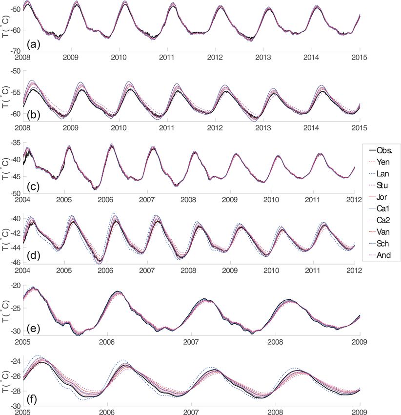
4202       M. Ding et al.: Evaluation of density-dependent empirical snow conductivity relationships in East Antarctica

ters such as snow density (e.g., Yen, 1981; Sturm et al., 1997;
Calonne et al., 2011).
   Density-dependent thermal conductivity relationships are
widely used in various model studies. For example, the em-
pirical relationship developed by Jordan (1991) was adopted
by the CLM land model, the SNTHERM snow model, and
many land surface energy balance studies, such as Wang et
al. (2017). Lecomte et al. (2013) used the relationships in
Yen (1981) and Sturm et al. (1997) for large-scale sea-ice–
ocean coupling models. Applying the density-dependent re-
lationship in Calonne et al. (2011), Hills et al. (2018) investi-
gated the heat transfer characteristics in the Greenland abla-
tion zone. Steger et al. (2017) analyzed the melt water reten-
tion in the Greenland ice sheet by adopting the snow density–
conductivity relationship given in Anderson (1976). Char-
alampidis (2016) used the relationship in Sturm et al. (1997)
to trace the retained meltwater in the accumulation area of
the southern Greenland ice sheet. However, none of those re-
lationships have been carefully validated by in situ data in
Antarctica ice sheets.
                                                                    Figure 1. The locations of Dome Argus, Eagle, and LGB69 in
   In this paper, firn temperature data and snow density pro-       Antarctica.
files from three sites in East Antarctica were chosen to vali-
date the applicability of these density–conductivity relation-
ships (Table S1). We first describe the meteorological obser-       from ∼ 400 to 500 kg m−3 from the surface to 10 m depth
vations. After introducing the method for validating the em-        (Fig. S1). EAGLE (76◦ 250 S; 77◦ 010 E) is a typical “surface
pirical density–conductivity relationships, we then present         glazed” area with a hard snow crust due to the effect of drift
the validation results, followed by discussions and conclu-         snow. Its snow accumulation is 10 cm w.e. yr−1 (30 cm snow-
sions.                                                              fall), the snow density increases from ∼ 380 to 550 kg m−3
                                                                    from the surface to 10 m (Fig. S2) depth, and the mean annual
                                                                    air temperature is approximately −40.80 ◦ C. Dome Argus
2   Site and observational description                              (80◦ 220 S, 70◦ 220 E; 4093 m a.s.l.) is the highest point of the
                                                                    east Antarctic ice sheet. It is also the summit of the ice divide
Several solar-powered automatic weather stations (AWSs)             of the Lambert Glacier drainage basin, ∼ 1248 km from the
have been deployed along a traverse route from Zhongshan            nearest coast, and the surrounding region has a surface slope
to Dome A within the cooperative framework between Chi-             of only 0.01 % or less. Dome Argus has an extremely low sur-
nese and Australian Antarctic programs. These include de-           face air temperature (annual mean of −52.1 ◦ C), specific hu-
ployments at LGB69 (in January 2002) and at EAGLE and               midity, and snow accumulation rate (around 2 cm w.e. yr−1 ),
Dome A (in January 2005). For more than 10 years since              and it experiences no surface melt, even at the peak of sum-
then, near-hourly meteorological measurements of air and            mer (Ding et al., 2016). The surface snow is very soft here,
firn temperature (at several heights and depths), relative hu-      and it ranges from ∼ 270 to 450 kg m−3 in the top 10 m
midity, wind, and air pressure have been made. The data             (Fig. S3). No radiation measurements were carried out at the
from the AWSs are collected remotely and relayed by the             site; therefore, it is nearly impossible to build a complete en-
ARGOS satellite transmission system. Firn temperatures are          ergy balance model at the snow surface of Dome Argus.
measured (using FS23D thermistors in a ratiometric circuit
with a resolution of 0.02K) at four depths below the surface;
                                                                    3     Methods
these were 0.1, 1, 3, and 10 m when deployed, but they have
slowly deepened with time due to snow accumulation. Due             3.1    Numerical model method
to heavy snowfall at LGB69, these data are only available for
2002–2008.                                                          We validate the heat conductivity by a 1D transient heat dif-
   All three sites are located on the western side of the Lam-      fusion model:
bert Glacier basin. LGB69 (70◦ 500 S, 77◦ 040 E; 1854 m a.s.l.)
                                                                    ∂T    K ∂ 2T
is only 192 km from the coast (Fig. 1) and has an annual pre-          =           ,                                             (1)
cipitation of 20 cm w.e. yr−1 (∼ 50 cm snowfall), strong wind       ∂t   Cs ρs ∂z2
(∼ 8.5 m s−1 annual), and a mean annual air temperature             where T is the firn temperature, K is the heat conductivity,
of approximately −26.10 ◦ C. The snow density increases             Cs is the heat capacity of snow, ρs is the density of snow,

The Cryosphere, 15, 4201–4206, 2021                                                     https://doi.org/10.5194/tc-15-4201-2021
M. Ding et al.: Evaluation of density-dependent empirical snow conductivity relationships in East Antarctica 4203
and z is the depth below the snow surface. The vertical firn in Table 1. At Dome A, the Jor and Sch relationships give
density profiles for three sites are shown in Figs. S1–S3. The us a significant discrepancy between observed and modeled
heat capacity of snow is estimated by assuming snow is a firn temperature (Fig. 2). The modeled firn temperature cal-
mixture of air and ice: culated by the Ca1, Lan, and Van relationships show a closer
agreement with the observed firn temperature. The density-
ρs ρs
Cs = Ci + Ca 1 − , (2) and temperature-dependent relationship, Ca2, however, does
ρi ρi not appear to have a better performance than its density-
where Ci and Ca are heat capacity of ice and air, respectively. dependent version Ca1 at Dome A.
We constrain the upper and lower model domain using two In Fig. 2 and Table 1, we can see that the Lan relation-
Dirichlet boundary conditions, the 0.1 and 10 m firn temper- ship gives the best performance at the depth of 1 and 3 m at
atures. The observed and modeled firn temperatures at the Dome A, followed by the Van and Ca1 relationships. The Lan
depths of 1 and 3 m are then compared over a period of time. relationship was derived from in situ snow conductivity mea-
The performance of different heat conductivity relationships surements on Filchner ice shelf (Lange, 1985). It is the only
is then evaluated by the deviation metric of the difference relationship in this study that is based on in situ firn sam-
between the modeled and observed temperature data: ple measurements in Antarctica. The Ca1 relationship was
derived by analyzing a wide range of different snow samples
N
1 X from a number of different geographical locations with many
σ2 = (Td − Tdm ), (3) different snow types (Calonne et al., 2011). The Van relation-
N i
ship is old but is adopted in Cuffey and Paterson (2010) and
still shows a nice performance in our model results.
where Td = abs(Tmodel − Tobs ), Tdm is the mean value of Td ,
Similarly to the Dome A case, at the Eagle station, the Ca1
and N is the number of the temperature dataset.
relationship outperforms other relationships, followed by the
3.2 Temperature phase-change method Ca2 and Yen relationships. The Jor, Stu, and Lan relation-
ships, however, appear not to be suitable for parameterizing
In this approach, we approximate the annual temperature cy- the firn conductivity, compared with other relationships at the
cles as sinusoidal functions (Demetrescu et al., 2007): Eagle station. At LGB69, however, the Sch and Jor relation-
ships appear to be superior to other relationships, in contrast
T (z, t) = Tm + A (z) sin (ω · t + φ (z)) , (4) to the cases at Dome A. The Jor relationship is based on
the experimental measurements in Yen (1962). Sch is also an
where T is the firn temperature expressed as a function of experimental relationship based on the data given in Mellor
depth z and time t, Tm is the mean annual value of T , A is (1977). In this case, the Ca2 relationship also gives a smaller
the amplitude of the annual firn temperature cycle, ω is the temperature difference compared with the Ca1 result. Note
frequency of the temperature cycle, and φ is the wave phase that the same relationship may show different performance
of the annual cycle. for different depth ranges. For example, for the Lan relation-
While it is common to fit a harmonic series (Fourier anal- ship, the modeled and observed firn temperature shows very
ysis) rather than a single sine wave to temperature variations, good agreement at a depth of 3 m but has a relatively large
we found that this gave no advantage over Eq. (4) for the discrepancy at a depth of 10 m.
data at the three sites because the temperature at the sites We also estimate the spatially averaged annual mean ther-
shows nonperiodic temperature excursions during the “core- mal conductivity from the temperature phase shifts between
less” Antarctic winter. Assuming the snow is horizontally the depth ranges of 0.1–1, 1–3, and 3–10 m at the Dome A
isotropic, we can estimate the apparent thermal diffusion, ka , (Fig. S4), Eagle (Fig. S5), and LGB69 (Fig. S6) stations,
from the changes in phase at different depths: and we compare them with the mean values corresponding to
different density–conductivity relationships (Table S2). The
ω (z2 − z1 )2 phase at different levels (φfit ) (also the phase shift, 1φfit ) is
ka = . (5)
2 (φ1 − φ2 )2 determined from the least squares fit to Eq. (1), and the ther-
mal diffusivity (conductivity) is then calculated using Eq. (5).
The conductivity can then be recovered from ka and the heat
Clearly, we can see that there is an increasing trend of con-
capacity of firn.
ductivity with depth (Table S2). Similar to the case in Ta-
ble 1, the Ca1 and Ca2 relationships give closer values than
4 Results and discussions the conductivity values recovered from the phase-change
method at the three different depth intervals, which is con-
In Figs. S4, S5, and S6, we show the comparisons of ob- sistent with the comparison results in Table 1. The Lan, Van,
served and modeled firn temperature using nine different and Yen relationships also show closer agreement with the
density–conductivity relationships at the Dome A, Eagle, and phase-change results. However, we do not see a consistent
LGB69 AWSs. The deviations of their differences are given pattern for the performance of different empirical density–
https://doi.org/10.5194/tc-15-4201-2021 The Cryosphere, 15, 4201–4206, 20214204 M. Ding et al.: Evaluation of density-dependent empirical snow conductivity relationships in East Antarctica
Table 1. Deviation (σ 2 ) of |Tmodel − Tobs | (K) for different density-dependent empirical relationships at 1 and 3 m for three stations. The
three overall best relationships for different depths are shown using “*”.
Yen Ca1 Jor Stu Lan Van Sch Ca2 And
1m 0.64 0.55* 0.91 0.44 0.30* 0.49* 0.92 0.67 0.70
Dome A
3m 0.46 0.35* 0.87 0.57 0.18* 0.28* 0.90 0.50 0.55
1m 0.33 0.36 0.22* 0.56 0.04* 0.44 0.19* 0.34 0.30
LGB69
3m 0.28 0.31 0.12* 0.57 0.39* 0.43 0.08* 0.13 0.23
1m 0.34* 0.32* 0.43 0.38 0.38 0.31 0.46 0.32* 0.36
Eagle
3m 0.14* 0.12* 0.33 0.38 0.69 0.19 0.39 0.13* 0.14
Yen refers to Yen (1981); Ca1 refers to Calonne et al. (2011); Jor refers to Jordan (1991); Stu refers to Sturm et al. (1997);
Lan refers to Lange (1985); Van refers to Van Dusen and Washburn (1929); Sch refers to Schwander et al. (1997); Ca2 refers
to Calonne et al. (2019); And refers to Anderson (1976).
Figure 2. Comparison of observed and modeled temperatures using different density-dependent conductivity relationships at depths of 1 m (a,
c, e) and 3 m (b, d, f) at Dome A (a, b), Eagle (c, d), and LGB69 (e, f).
conductivity relationships. At different depth levels, differ- and ice (Eq. 2). In addition, only one relationship is a func-
ent relationships appear to show varying model performance. tion of firn temperature (Ca2). As temperature is an impor-
This is possibly a result of our assumption that the vertical tant parameter affecting firn heat conductivity (Calonne et
density profile is kept constant in time and that the heat ca- al., 2019), considering only density in the other eight rela-
pacity of firn is a linear relationship of the capacity of air tionships may introduce model uncertainties in our evalua-
The Cryosphere, 15, 4201–4206, 2021 https://doi.org/10.5194/tc-15-4201-2021M. Ding et al.: Evaluation of density-dependent empirical snow conductivity relationships in East Antarctica 4205
tion. However, as we consider a long time span of observa- Disclaimer. Publisher’s note: Copernicus Publications remains
tion and model years (7 years for Dome A, 8 years for Eagle, neutral with regard to jurisdictional claims in published maps and
and 3 years for LGB69), the overall deviation of modeled and institutional affiliations.
observed temperature should be accountable for quantifying
the performance of different density-dependent conductivity
relationships. Acknowledgements. The observations in Antarctica were logisti-
cally supported by the Chinese National Antarctic Research Expe-
dition (CHINARE).
5 Conclusions Financial support. This Research has been supported by
the National Natural Science Foundation of China (grant
no. 42122047), the National Key R&D Program of China (grant
In this study, we apply two methods to validate nine differ- no. 2019YFC1509100), and the Basic Fund of the Chinese
ent density–conductivity relationships: (1) by applying a 1D Academy of Meteorological Sciences (grant nos. 2021Z006 and
vertical heat diffusivity model, we compare the modeled firn 2019Z008).
temperature at a depth of 1 and 3 m with observations; (2) we
compare the mean empirical snow conductivity at three depth
intervals (0.1–1, 1–3, and 3–10 m) according to the phase- Review statement. This paper was edited by Adam Booth and re-
change-derived temperature variations. viewed by two anonymous referees.
It is found that some empirical density relationships have
generally good model performance and agree well with
phase-change-recovered conductivity, but they show diverse References
behaviors at different depth levels. Based on these two meth-
ods, we find that the relationship proposed by Calonne et Anderson, E. A.: A Point Energy and Mass Balance Model of
al. (2011) (Ca1) generally has the best overall performance. a Snow Cover, Technical Report, National Weather Service,
United States, 1976.
The Jordan (1991) relationship (used in snow models like
Calonne, N., Flin, F., Morin, S., Lesaffre, B., Rolland du Roscoat,
CLM and SNTHERM), however, does not present very good S., and Geindreau, C.: Numerical and experimental investiga-
model results for Dome A, Eagle, or LGB69. All in all, no tions of the effective thermal conductivity of snow, Geophys.
density–conductivity relationship is optimal at all sites, and Res. Lett., 38, 537–545, https://doi.org/10.1029/2011GL049234,
the performance of each varies with depth. 2011.
The three AWS sites in the paper cover a large range of el- Calonne, N., Milliancourt, L., Burr, A., Philip, A., Mar-
evation and distances from the coast. Thus, we argue that our tin, C. L., Flin, F., and Geindreau, C.: Thermal conduc-
findings can shed some lights on firn thermal studies (e.g., tivity of snow, firn, and porous ice from 3-D image-
the applicability of different firn density–conductivity rela- based computations, Geophys. Res. Lett., 46, 13079–13089,
tionships) in Antarctica. https://doi.org/10.1029/2019GL085228, 2019.
Charalampidis, C., Van As, D., Colgan, W. T., Fausto, R.
S., Macferrin, M., and Machguth, H.: Thermal tracing of
retained meltwater in the lower accumulation area of the
Data availability. AWS data are publicly available from
Southwestern Greenland ice sheet, Ann. Glaciol., 57, 1–10,
https://doi.org/10.26179/brjy-g225 (Heil et al., 2017),
https://doi.org/10.1017/aog.2016.2, 2016.
https://doi.org/10.11856/SNS.D.2021.006.v0 (Ding et al., 2021a),
Cuffey, K. M. and Paterson, W. S. B.: The physics of glaciers, 4th
and https://doi.org/10.11856/SNS.D.2021.007.v0 (Ding et al.,
edn., Butterworth-Heinemann, Oxford, 2010.
2021b).
Demetrescu, C., Nitoiu, D., Boroneant, C., Marica, A., and Lu-
caschi, B.: Thermal signal propagation in soils in Romania: con-
ductive and non-conductive processes, Clim. Past, 3, 637–645,
Supplement. The supplement related to this article is available on- https://doi.org/10.5194/cp-3-637-2007, 2007.
line at: https://doi.org/10.5194/tc-15-4201-2021-supplement. Ding, M., Xiao, C., Yang, Y., Wang, Y., Li, C., Yuan, N., Shi, G.,
Sun, W., and Ming, J.: Re-assessment of recent (2008-2013) sur-
face mass balance over Dome Argus, Antarctica, Polar Res., 35,
Author contributions. MD designed and wrote the paper; TZ un- 26133, https://doi.org/10.3402/polar.v35.26133, 2016.
dertook the calculation; DY and IA processed the AWS data; TD Ding, M., Yang, D., van den Broeke, M. R., Allison, I., Xiao, C.,
and CX evaluated the paper. All authors contributed to editing the Qin, D., and Huai, B.: The surface energy balance at Panda 1 Sta-
paper. tion, Princess Elizabeth Land: a typical katabatic wind region in
East Antarctica, J. Geophys. Res.-Atmos., 125, e2019JD030378,
https://doi.org/10.1029/2019JD030378, 2020.
Competing interests. The authors declare that they have no conflict Ding, M., Zhang, T., and Allison, I.: Automatic Weather
of interest. Station Data obtained at EAGLE, Antarctica, Na-
https://doi.org/10.5194/tc-15-4201-2021 The Cryosphere, 15, 4201–4206, 20214206 M. Ding et al.: Evaluation of density-dependent empirical snow conductivity relationships in East Antarctica tional Arctic and Antarctic Data Center [data set], Riche, F. and Schneebeli, M.: Thermal conductivity of snow mea- https://doi.org/10.11856/SNS.D.2021.006.v0, 2021a. sured by three independent methods and anisotropy considera- Ding, M., Zhang, T., and Allison, I.: Automatic Weather tions, The Cryosphere, 7, 217–227, https://doi.org/10.5194/tc-7- Station Data obtained at LGB69, Antarctic a, Na- 217-2013, 2013. tional Arctic and Antarctic Data Center [data set], Schwander, J., Sowers, T., Barnola, J. M., Blunier, T., Fuchs, A., and https://doi.org/10.11856/SNS.D.2021.007.v0, 2021b. Malaizé, B.: Age scale of the air in the summit ice: Implication Dutra, E., Balsamo, G., Viterbo, P., Miranda, P. M. A., Bel- for glacial-interglacial temperature change, J. Geophys. Res., jaars, A., Schär, C., and Elder, K.: An Improved Snow 102, 19483–19493, https://doi.org/10.1029/97JD01309, 1997. Scheme for the ECMWF Land Surface Model: Descrip- Sergienko, O. V., Macayeal, D. R., and Thom, J. E.: Reconstruc- tion and Offline Validation, J. Hydrometeor., 11, 899–916, tion of snow/firn thermal diffusivities from observed tempera- https://doi.org/10.1175/2010JHM1249.1, 2010. ture variation: application to iceberg C16, Ross Sea, Antarctica, Heil, P., Hyland, G., and Alison, I.: Automatic Weather Station 2004–07, Ann. Glaciol., 49, 91–95, 2008. Data obtained at Dome A (Argus), Antarctica, Ver. 1, Australian Steger, C. R., Reijmer, C. H., van den Broeke, M. R., Wever, N., Antarctic Data Centre [data set], https://doi.org/10.26179/brjy- Forster, R. R., Koenig, L. S., Kuipers Munneke, P., Lehning, M., g225, 2017. Lhermitte, S., Ligtenberg, S. R., and Miège, C.: Firn meltwater Hills, B. H., Harper, J. T., Meierbachtol, T. W., Johnson, J. V., retention on the Greenland ice sheet: A model comparison, Front. Humphrey, N. F., and Wright, P. J.: Processes influencing heat Earth Sci., 5, 3, https://doi.org/10.3389/feart.2017.00003, 2017. transfer in the near-surface ice of Greenland’s ablation zone, The Sturm, M., Holmgren, J., König, M., and Morris, K.: The ther- Cryosphere, 12, 3215–3227, https://doi.org/10.5194/tc-12-3215- mal conductivity of seasonal snow, J. Glaciol., 43, 26–41, 2018, 2018. https://doi.org/10.3189/S0022143000002781, 1997. Hurley, S. and Wiltshire, R. J.: Computing thermal diffusivity from Van Dusen, M. S. and Washburn, E. W.: Thermal conductivity soil temperature measurements, Comput. Geosci., 19, 475–477, of non-metallic solids, International critical tables of numerical https://doi.org/10.1016/0098-3004(93)90096-N, 1993. data, physics, chemistry and technology, New York, McGraw- Jordan, R.: A One-Dimensional Temperature Model for a Snow Hill, 5, 216–217, 1929. Cover: Technical Documentation for SNTHERM, 89, U.S. Army Wang, L., Zhou, J., Qi, J., Sun, L., Yang, K., Tian, L., Lin, Cold Regions Research and Engineering Laboratory, Hanover, Y., Liu, W., Shrestha, M., Xue, Y., and Koike, T.: Devel- NH, USA, 1991. opment of a land surface model with coupled snow and Lange, M. A.: Measurements of thermal parameters in frozen soil physics, Water Resour. Res., 53, 5085–5103, Antarctic snow and firn, Ann. Glaciol., 6, 100–104, https://doi.org/10.1002/2017WR020451, 2017. https://doi.org/10.3189/1985AoG6-1-100-104, 1985. Yen, Y. C.: Effective thermal conductivity of ven- Lecomte, O., Fichefet, T., Vancoppenolle, M., Domine, F., Mas- tilated snow, J. Geophys. Res., 67, 1091–1098, sonnet, F., Mathiot, P., Morin, S. and Barriat, P. Y.: On https://doi.org/10.1029/JZ067i003p01091, 1962. the formulation of snow thermal conductivity in large-scale Yen, Y. C.: Review of Thermal Properties of Snow, Ice and Sea Ice, sea ice models, J. Adv. Model. Earth Sy., 5, 542–557, U.S. Army Cold Regions Research and Engineering Laboratory, https://doi.org/10.1002/jame.20039, 2013. United States, 27 pp., Crrel Report No: CR, 81-10, 1981. Mellor, M.: Engineering properties of snow, J. Glaciol., 19, 15–66, 1977. Oldroyd, H. J., Higgins C. W., Huwald, H., Selker, J. S., and Par- lange, M. B.: Thermal diffusivity of seasonal snow determined from temperature profiles, Adv. Water Resour., 55, 121–130, https://doi.org/10.1016/j.advwatres.2012.06.011, 2013. The Cryosphere, 15, 4201–4206, 2021 https://doi.org/10.5194/tc-15-4201-2021
You can also read