Denoising High-field Multi-dimensional MRI with Local Complex PCA - bioRxiv
←
→
Page content transcription
If your browser does not render page correctly, please read the page content below
bioRxiv preprint first posted online Apr. 11, 2019; doi: http://dx.doi.org/10.1101/606582. The copyright holder for this preprint
     (which was not peer-reviewed) is the author/funder, who has granted bioRxiv a license to display the preprint in perpetuity.
                                       It is made available under a CC-BY 4.0 International license.

 1                     Denoising High-field Multi-dimensional MRI with Local Complex PCA
 2
 3         Pierre-Louis Bazin1,2, Anneke Alkemade1, Wietske van der Zwaag3, Matthan Caan4, Martijn
 4                                       Mulder1,5, Birte U. Forstmann1
 5
 6        1 Integrative
                      Model-based Cognitive Neuroscience research unit, Universiteit van Amsterdam,
 7       Amsterdam, The Netherlands; 2 Max-Planck Institute for Human Cognitive and Brain Sciences,
 8        Leipzig, Germany; 3 Spinoza Centre for Neuroimaging, Amsterdam, The Netherlands; 4 Brain
 9          Imaging Centre, Amsterdam University Medical Center, Amsterdam, The Netherlands; 5
10                  Psychology Department, Universiteit Utrecht, Utrecht, The Netherlands
11
12
13                                                Abstract
14    Modern high field and ultra high field magnetic resonance imaging (MRI) experiments routinely
15    collect multi-dimensional data with high spatial resolution, whether multi-parametric structural,
16    diffusion or functional MRI. While diffusion and functional imaging have benefited from recent
17    advances in multi-dimensional signal analysis and denoising, structural MRI has remained
18    untouched. In this work, we propose a denoising technique for multi-parametric quantitative MRI,
19    combining a highly popular denoising method from diffusion imaging, over-complete local PCA,
20    with a reconstruction of the complex-valued MR signal in order to define stable estimates of the
21    noise in the decomposition. With this approach, we show signal to noise ratio (SNR) improvements
22    in high resolution MRI without compromising the spatial accuracy or generating spurious
23    perceptual boundaries.
24
25
26    1. Introduction
27
28    Ultra-high field magnetic resonance (MR) imaging at 7 Tesla and beyond has enabled
29    neuroscientists to probe the human brain in vivo beyond the macroscopic scale (Weiskopf et al.,
30    2015). In particular, quantitative MRI techniques (Cercignani et al., 2018) have become more
31    readily available and offer the promise of quantitative information about the underlying
32    microstructure. Unfortunately, as the size of the imaging voxel decreases well below the cubic
33    millimeter, so does the signal to noise ratio (SNR), and the achievable resolution even when
34    imaging a small portion of the brain remains limited, and requires multiple averages at the highest
35    resolutions (Fedeeau et al., 2018; Fracasso et al., 2016; Stucht et al., 2015).
36             Multi-parametric quantitative methods acquire multiple images within a single sequence, in
37    order to estimate the underlying quantity (Helms et al. 2008, Metere et al. 2017, Caan et al., 2018).
38    This is comparable to diffusion-weighted MR imaging (DWI) where multiple images with different
39    weighting are acquired. Recent work in diffusion analysis demonstrated that the intrinsic
40    redundancy of the signal across these images can be employed to separate signal from noise with a
41    principal component analysis (PCA) over small patches of the images (Manjon et al., 2013; Veraart
42    et al., 2016). This principle can be transferred to multi-parametric quantitative MRI: in this work we
43    present an extension of the PCA denoising to the recently described MP2RAGEME sequence,
44    which provides estimates of R1 and R2* relaxation rates as well as quantitative susceptibility maps
45    (QSM) in a very compact imaging sequence (Caan et al., 2018).
46             The MP2RAGEME data comes with additional challenges for the classical PCA approaches.
47    First, the images are complex-valued, comprising of both magnitude and phase needed for the
48    estimation of quantitative MRI parameters. This complex nature of the data needs to be taken into
49    account. Second, they include only a few images compared to the high number of directions
50    acquired in DWI. Interestingly, we can make fairly simple assumptions about the dimensionality of

                                                                            1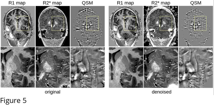
bioRxiv preprint first posted online Apr. 11, 2019; doi: http://dx.doi.org/10.1101/606582. The copyright holder for this preprint
      (which was not peer-reviewed) is the author/funder, who has granted bioRxiv a license to display the preprint in perpetuity.
                                        It is made available under a CC-BY 4.0 International license.

 51    the signal, as it contains primarily R1, R2*, susceptibility and proton density (PD) weighting.
 52    Taking these features into account, we were able to effectively denoise high resolution
 53    MP2RAGEME data without averaging, and maintain spatial precision. We studied the impact of
 54    denoising on the computation of quantitative maps, and its practical impact for delineating small,
 55    low contrast subcortical nuclei such as the habenula, a notoriously difficult small nucleus in the
 56    subcortex.
 57
 58
 59    2. Materials and Methods
 60
 61    2.1. Data acquisition
 62    Our denoising method focuses on the recently developed MP2RAGEME sequence (Caan et al.,
 63    2018) which combines multiple inversions and multiple echoes from a magnetisation-prepared
 64    gradient echo sequence (MPRAGE) to simultaneously obtain an estimate of quantitative T1, T2*
 65    and susceptibility. The specific protocol of interest is comprised of five different images: a first
 66    inversion with T1 weighting, followed by a second inversion with predominantly PD weighting and
 67    four echoes with increasing T2* weighting (Fig. 1).
 68
 69
 70    Figure 1: The MP2RAGEME sequence: A: first inversion, B,D,C,E: second inversion, first to fourth
 71    echo (top: magnitude, bottom: phase).
 72
 73
 74    For the experiments, we used a high-resolution imaging slab centered on the subcortex with the
 75    following parameters: resolution = 0.5mm isotropic, TR = 8.33s, TR1 = 8ms, TR2 = 32ms, TE1 =
 76    4.6ms, TE2A-D = 4.6/12.6/20.6/28.6ms, TI1/TI2 = 670/3738ms, α1/α2 = 7/8o. Data was obtained for
 77    five healthy human subjects as part of an ongoing atlasing study approved by the Ethics Review
 78    Board of the Faculty of Social and Behavioral Sciences, University of Amsterdam, The Netherlands
 79    (approval number: 2016-DP-6897). All subjects provided written informed consent for the study.
 80
 81
 82    2.2. Complex signal reconstruction
 83    One of the main drawbacks of existing local PCA methods for denoising is that they work on
 84    magnitude images, which follow Rician distributions. A simple correction proposed in (Eichner et
 85    al., 2016) for removing the Rician bias in DWI averaging is to revert to the complex signal, taking
 86    into account the phase information. Phase contains additional variations due to non-local effects of
 87    air cavities around the brain, which bring severe ringing artifacts in the reconstructed data (Fig.2A).
 88    In (Eichner et al., 2016), the global phase information is removed with a total variation method,
 89    which generally respects the location of phase wraps. However, we found that this approach is not
 90    effective in regions where the phase wraps have high frequency, and there are residual phase
 91    artifacts in the local phase. While these have little consequences for their averaging application,
 92    they provide systematic variations for the PCA decomposition, which is undesirable here. We
 93    therefore start with a full phase unwrapping (Abdul-Rahman et al., 2005) followed by a total
 94    variation smoothing (Chambolle, 2004) of the unwrapped phase (Fig.2B). The residual phase
 95    variations are used as local phase, and combined with the magnitude to reconstruct real and
 96    imaginary parts of the complex signal (Fig.2C,D). Note that here, unlike (Eichner et al., 2016), we
 97    do not discard the imaginary part of the signal as it contains valuable information about the noise
 98    and residual anatomical information.
 99
100

                                                                             2
bioRxiv preprint first posted online Apr. 11, 2019; doi: http://dx.doi.org/10.1101/606582. The copyright holder for this preprint
      (which was not peer-reviewed) is the author/funder, who has granted bioRxiv a license to display the preprint in perpetuity.
                                        It is made available under a CC-BY 4.0 International license.

101    Figure 2: Phase preprocessing. A: original phase map, B: after unwrapping and global
102    phase removal, C: reconstructed real signal, D: reconstructed imaginary signal.
103
104
105    2.3. Local PCA of complex signal
106    The complex signal, now comprising ten images all similar in nature, is then processed following
107    the local overcomplete PCA approach of (Manjón et al., 2013). In short, the images are cut into
108    small, overlapping patches of NxNxN voxels, and the M contrasts combined into a N3xM matrix.
109    The average patch value per contrast is subtracted, and the matrix decomposed via singular value
110    decomposition (SVD) to yield the eigenvectors and associated singular values (square roots of the
111    eigenvalues) of the covariance matrix across the patch. In this work, we used patches of size N = 4,
112    and M = 10.
113            The overlapping patches are combined following the technique of (Manjón et al., 2013),
114    weighting each patch by the number of kept eigenvectors                         . Once recombined, the
115    eigenvectors rapidly change from a rich information content, encoding boundaries, to pure noise
116    (Fig. 3). However, the decision boundary between actual signal and noise is variable across the
117    brain, due to the presence of different tissue types, multiple tissue boundaries, etc. In order to infer
118    for each patch the number of eigenvectors to keep, we thus need to first quantify the expected noise
119    distribution over the SVD.
120
121
122    Figure 3: Local PCA decomposition: first five eigenvectors (top) and singular values
123    (bottom) from highest to lowest.
124
125
126    2.4. Estimating the noise
127    Noise estimation in advanced MRI is far challenging: variations in coil sensitivity, non-local
128    susceptibility effects and dependencies to the B0 field as well as various acquisition techniques will
129    affect the signal and the noise differently in different regions. The original local PCA denoising
130    methods of (Manjón et al., 2013) used elaborate estimates of the magnitude image noise, taking into
131    account its Rician properties. A recent extension of the work fit the expected distribution of
132    eigenvalues from a random Rician noise matrix to determine its threshold (Veraart et al., 2016).
133             In this work, we propose a simpler approach based on two properties of the complex signal:
134    first, that the noise is locally Gaussian, and second that the spread of singular values for Gaussian
135    noise can be reasonably well approximated by a straight line (Fig.4A,B). In addition, this simple
136    property is retained by interpolation (Fig.4C,D), which makes it possible to perform denoising after
137    image registration, for instance when motion correction is needed as in DWI or fMRI, or after fat
138    navigator-based motion correction in structural MRI (Gallichan and Marques, 2017).
139
140
141    Figure 4: Noise properties of the singular value decomposition (SVD). A: SVD of 15 simulated
142    4x4x4 voxel Gaussian noise patterns, B: Distribution of R2 residuals over from fitting a line to the
143    second half of 100,000 simulated noise patterns, C: SVD of 15 simulated 4x4x4 voxel Gaussian
144    noise patterns after a random sub-voxel shift and trilinear interpolation, D: Distribution of R2
145    residuals for 100,000 simulated noise patterns with the same random shift, E: Map of estimated
146    number of kept eigenvectors from actual data, F: Map of the fitting R2 residuals, G: Map of kept
147    eigenvectors after co-registration and trilinear interpolation of the data, H: Map of the fitting R2
148    residuals after co-registration.
149
150

                                                                             3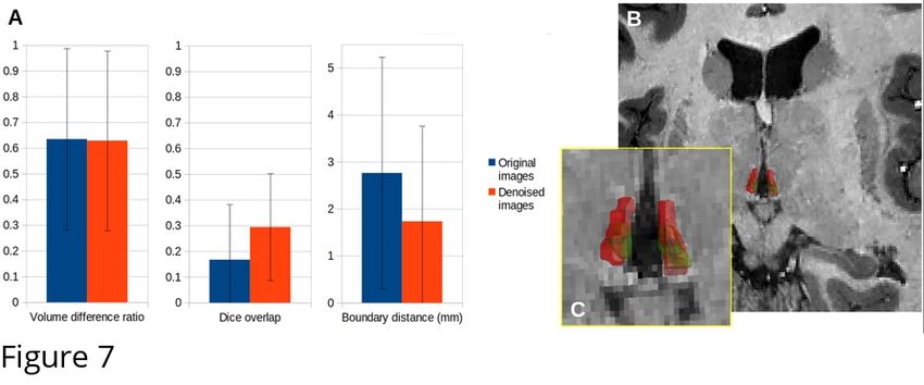
bioRxiv preprint first posted online Apr. 11, 2019; doi: http://dx.doi.org/10.1101/606582. The copyright holder for this preprint
(which was not peer-reviewed) is the author/funder, who has granted bioRxiv a license to display the preprint in perpetuity.
It is made available under a CC-BY 4.0 International license.
151 Our algorithm to estimate the noise level proceeds as follows. First, a line is fitted to the M/2
152 = 5 lowest singular values of the patch decomposition using linear least squares. Then, every
153 singular value above a factor of α above the expected noise level given by the fitted line is kept,
154 while the others are removed. Thus, the main requirements of our method are that: 1) local signal
155 variations across contrasts in each individual patch are Gaussian-distributed, and 2) the intrinsic
156 dimension of the data is lower than half of the number of acquired images. The patches are then
157 reconstructed and averaged across the image, the complex images separated into magnitude and
158 phase, and finally the discarded global phase variations are reintroduced and wrapped, to obtain
159 data as similar as possible to the original input. In addition, a map of the number of kept
160 eigenvectors and of the noise fitting residuals weighted by patch are computed for quality control
161 (Fig.4E,F,G,H). The complete denoising algorithm is available in Open Source as part of the IMCN
162 Toolkit (https://www.github.com/imcn-uva/imcn-imaging/) and the Nighres library (Huntenburg et
163 al., 2018; https://www.github.com/nighres/nighres/).
164
165
166 2.5. Quantitative Mapping
167 The main interest of quantitative MR mapping techniques such as the MP2RAGEME sequence is to
168 obtain estimates of the MR parameters of T1, T2* relaxation times and susceptibility χ from the
169 measured images. In order to do so, we used the look-up table method of (Marques et al., 2010) to
170 generate T1 estimates, a simple regression in log domain to obtain T2* (Miller and Joseph, 1993)
171 and the TGV-QSM reconstruction algorithm of (Langkammer et al., 2015) to create quantitative
172 susceptibility maps (QSM), following the approach of (Caan et al., 2018) to estimate QSM for each
173 of the three last echoes of the second inversion and take the median. T1 and T2* mapping methods
174 are included in the Nighres library, and the TGV-QSM algorithm is also freely available
175 (http://www.neuroimaging.at/pages/qsm.php).
176
177
178 2.6. Manual delineations
179 In order to obtain structure-specific measures of quality and to evaluate the practical benefits of the
180 method for segmentation purposes, we performed a manual segmentation study. To evaluate the
181 benefits of the denoising, we selected the habenula, a small and challenging structure ventral to the
182 thalamus, which together with the pineal gland and stria medullaris form the epithalamus (Mai et al,
183 2016; Hikosaka, 2010; Strotmann et al., 2013). Since we cannot distinguish between the medial and
184 lateral habenula on MRI, both were included in our delineations. Given its size, complex shape, and
185 heterogeneous composition, the habenula requires high resolution images and detailed anatomical
186 knowledge to be reliably delineated on MRI.
187 In this study, the habenula was delineated by two raters on the reconstructed quantitative T1
188 maps obtained with or without denoising. The consensus mask (regions labeled by all raters on all
189 images) were used to measure noise properties, while the overlap of the masks was used to measure
190 inter-rater reliability.
191
192
193 2.7. Co-registration to standard space
194 Previously proposed methods for local PCA denoising have shown decreased performance when
195 handling interpolated data due to the changes in the noise distribution (Manjón et al., 2013; Veraart
196 et al., 2016). To test the performance of our noise estimation approach, we co-registered our data to
197 standard space by aligning it first with a whole brain image of the same subject and then to the
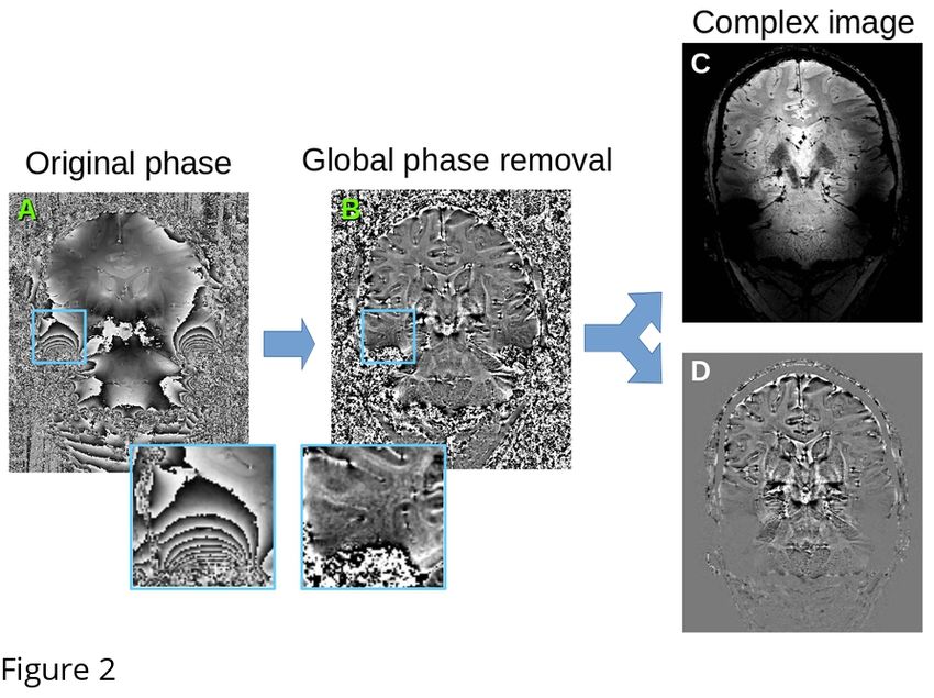
198 MNI152 template at 0.5 mm resolution. Both registrations used the first inversion of the
199 MP2RAGEME sequence, and were performed with linear registration in ANTS (Avants et al.,
4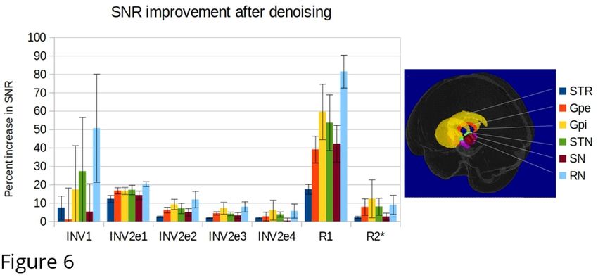
bioRxiv preprint first posted online Apr. 11, 2019; doi: http://dx.doi.org/10.1101/606582. The copyright holder for this preprint
      (which was not peer-reviewed) is the author/funder, who has granted bioRxiv a license to display the preprint in perpetuity.
                                        It is made available under a CC-BY 4.0 International license.

200    2008). Phase images were unwrapped before transformation to avoid interpolating across phase
201    wraps, and quantitative maps were computed before and after denoising in standard space.
202
203
204    2.8. Region labeling
205    Finally, to evaluate the signal improvement across a variety of structures, we used manual
206    delineations of the striatum, globus pallidus internal and external segment, subthalamic nucleus,
207    substantia nigra and red nucleus obtained from lower resolution MP2RAGEME images
208    (0.64x0.64x0.7 mm resolution) with higher SNR. The delineations were performed independently
209    by two raters and the conjunction between them was used as the structure mask. The masks were
210    co-registered linearly to the high resolution slab based on their scanner coordinates followed by a
211    rigid registration in ANTS. The intensities of the quantitative maps inside each region were used to
212    compute signal-to-noise ratio statistics of the original images and reconstructed quantitative maps
213    before and after denoising in original space.
214
215
216    3. Results
217
218    3.1. Impact on quantitative maps
219    As shown in Fig.5, the LCPCA denoising strongly impacts the estimation of quantitative signals, as
220    the SNR gains of multiple images are combined. Visually, we found a strong gain in particular for
221    R2* mapping, which is quite noise-sensitive with the low number of echo times of the
222    MP2RAGEME sequence. While the improvements are subtle at the whole brain scale, they are very
223    clear when focusing on small regions, particularly in the subcortex where the original SNR is low.
224
225
226    Figure 5: Comparison of quantitative MRI reconstruction: left, from the original MP2RAGEME
227    images; right from the denoised result.
228
229
230    3.2. SNR Measures
231    The denoising systematically improved the SNR in all structures, although not identically across
232    regions and contrasts (Fig.6). On individual MP2RAGEME images, the improvement was modest,
233    while denoising had a stronger cumulative impact on quantitative map estimation, especially for R1.
234    While R2* appears visually improved, the SNR measures were more similar partly due to the
235    heterogeneity of R2* values in many anatomical structures. QSM is the least affected, both visually
236    and quantitatively, which is expected as the quantitative susceptibility reconstruction algorithm
237    includes its own spatial regularization method (in this case, total generalized variation (TGV)). Still,
238    some more heterogeneous regions of the subcortex appear smoother after denoising. Interestingly,
239    the highest gains were obtained for the smaller structures such as substantia nigra, sub-thalamic
240    nucleus and red nucleus.
241
242
243    Figure 6: SNR improvement for the delineated structures and the different contrasts (from left to
244    right: first inversion, second inversion echo 1 to 4, estimated R1 map, estimated R2* map,
245    estimated QSM; mean and standard deviation across subjects).
246
247
248    3.3. Impact on manual delineations

                                                                             5
bioRxiv preprint first posted online Apr. 11, 2019; doi: http://dx.doi.org/10.1101/606582. The copyright holder for this preprint
(which was not peer-reviewed) is the author/funder, who has granted bioRxiv a license to display the preprint in perpetuity.
It is made available under a CC-BY 4.0 International license.
249 Manual delineations of the habenula are challenging, and inter-rater agreement is low. Our
250 denoising improved the consensus (Fig. 7), but not to the point of an acceptable level of
251 reproducibility for measuring anatomical quantities such as volume or shape.
252
253
254 Figure 7: Comparison of manual delineations of the lateral habenula with or without denoising. A:
255 Inter-rater agreement between delineations, B: 3D rendering of the lateral habenula in one subject,
256 as delineated by each rater (red and green outline, respectively), C: Inter-rater difference between
257 delineations and average internal contrast variations.
258
259
260 3.4. Effects of interpolation
261 When performing the denoising step after image co-registration to a standard space and
262 interpolation, we observe only small differences in the LCPCA algorithm behavior (Fig.4G,H). The
263 interpolation procedure tends to slightly increase the dimension of the kept signal, probably due to
264 the mixing of signals across voxels. However, the proposed dimensionality estimation procedure
265 appears largely robust to interpolation.
266
267
268 4. Discussion
269
270 In this work we presented a new local PCA denoising technique, using the full complex signal
271 acquired to correct acquisitions with multiple image contrasts such as DWI or quantitative MRI
272 sequences. Even with a sequence like MP2RAGEME, where only five different images are used in
273 order to recover T1, T2* and QSM, the proposed approach was able to effectively reduce the noise
274 without introducing blurring artifacts. The homogeneity of structures compared to their boundary
275 was improved over the basal ganglia structures, and delineation of small nuclei such as the habenula
276 was shown to be more reproducible in high resolution images with high levels
277 of imaging noise.
278 By using both magnitude and phase information, the proposed method captures the entire
279 noise distribution, and stays in the statistically simpler domain of Gaussian perturbations. However,
280 obtaining high quality phase images is not trivial for all scanners and imaging sequences and can be
281 a limitation also in retrospective processing, as the phase is commonly discarded. Note also that
282 certain acceleration techniques such as partial Fourier encoding may sacrifice the phase signal
283 estimation. While there is no conceptual requirement to use both phase and magnitude in the
284 denoising, lowering the number of dimensions reduces the applicability of the method: in the case
285 of the MP2RAGEME using only five dimensions in order to separate four-dimensional signals from
286 noise is challenging, and the linear fit of the noise to the last half of the local PCA eigenvalues
287 becomes unreliable. Yet, preliminary experiments with other relaxometry methods such as multi-
288 parameter mapping (Weiskopf et al., 2013), which acquire between 14 and 20 images, indicated that
289 the separation of signal and noise based on magnitude alone was possible (unpublished data).
290 The main requirements of the noise estimation method are that: 1) local signal variations
291 across contrasts in each individual patch are Gaussian-distributed, and 2) the intrinsic dimension of
292 the data is generally lower than half of the number of acquired images. The first requirement is
293 easily met in small patches, regardless of the type of data acquired. The second requirement
294 depends on the type of MR sequence and tissue properties under consideration, but can be met
295 simply by running twice the same sequence, as is commonly done for increasing SNR by classical
296 averaging. Note also that in the case of a single contrast the PCA approach reduces to simple
297 averaging with no added value.
6bioRxiv preprint first posted online Apr. 11, 2019; doi: http://dx.doi.org/10.1101/606582. The copyright holder for this preprint
(which was not peer-reviewed) is the author/funder, who has granted bioRxiv a license to display the preprint in perpetuity.
It is made available under a CC-BY 4.0 International license.
298 The main interest of the PCA-based approaches for denoising high resolution images is that
299 unlike most other methods, they do not impose spatial regularity but rather enforce regularity across
300 contrasts, preserving small anatomical details without blurring or inducing artificial boundaries. In
301 addition, while the impact of noise removal on conventional MR images remains subtle, it offers the
302 option to push MR sequences beyond the usually accepted limits of thermal noise as long as enough
303 signal remains to be reliably detected. As ultra-high field advances toward higher and higher
304 resolutions, such denoising methods may become essential part of the imaging protocol for multi-
305 contrast anatomical imaging in the same way they have become a standard tool for advanced DWI
306 pre-processing (Veraart et al., 2016).
307 Finally, the proposed method is generally applicable to other relaxometry sequences such as
308 multi-echo GRE, multi-echo MPRAGE or multi-parametric maps (MPM), as well as DWI or
309 (multi-echo) fMRI. Other types of MR sequences that include multiple images with different
310 contrast may benefit from this approach, as long as the total number of images is sufficient to
311 properly estimate noise properties.
312
313
314 Conclusions
315
316 Here we presented a new local PCA method to denoise high resolution multi-parametric
317 quantitative MRI data. Combining magnitude and phase data, we could differentiate between
318 signal- and noise-induced variations with a simple model that is robust to interpolation. The
319 resulting quantitative images are automatically regularized and additional anatomical detail is
320 visible in low contrast regions. The denoising software is openly available as part of the IMCN
321 Toolkit (https://www.github.com/imcn-uva/imcn-imaging/) and the Nighres library
322 (https://www.github.com/nighres/nighres/). The proposed method can be extended to denoise other
323 MR imaging sequences with similar properties, namely partially redundant contrasts and low
324 intrinsic dimensionality. While the method is already efficient to denoise MR images acquired with
325 cutting edge methods at the lower limits of SNR, we hope they may help further to push MR
326 imaging toward acquiring even more challenging data where the noise may visually dominate but
327 significant amounts of signal are still available.
328
329
330 References
331
332 Abdul-Rahman, H., Gdeisat, M., Burton, D., Lalor, M., 2005. Fast three-dimensional phase-
333 unwrapping algorithm based on sorting by reliability following a non-continuous path, in: Osten,
334 W., Gorecki, C., Novak, E.L. (Eds.), . Presented at the Optical Metrology, Munich, Germany, p. 32.
335 https://doi.org/10.1117/12.611415
336
337 Caan, M.W.A., Bazin, P., Marques, J.P., Hollander, G., Dumoulin, S., Zwaag, W., 2018.
338 MP2RAGEME: T 1 , T 2 * , and QSM mapping in one sequence at 7 tesla. Human Brain Mapping.
339 https://doi.org/10.1002/hbm.24490
340
341 Cercignani, M., Dowell, N.G., Tofts, P.S. (eds), 2018. Quantitative MRI of the Brain: Principles of
342 Physical Measurement, Second edition, 2018. . CRC Press. https://doi.org/10.1201/b21837
343
344 Chambolle, A., 2004. An algorithm for total variation minimization and applications. Journal of
345 Mathematical imaging and vision 20, 89–97.
346
7bioRxiv preprint first posted online Apr. 11, 2019; doi: http://dx.doi.org/10.1101/606582. The copyright holder for this preprint
(which was not peer-reviewed) is the author/funder, who has granted bioRxiv a license to display the preprint in perpetuity.
It is made available under a CC-BY 4.0 International license.
347 Eichner, C., Cauley, S.F., Cohen-Adad, J., Möller, H.E., Turner, R., Setsompop, K., Wald, L.L.,
348 2015. Real diffusion-weighted MRI enabling true signal averaging and increased diffusion contrast.
349 NeuroImage 122, 373–384. https://doi.org/10.1016/j.neuroimage.2015.07.074
350
351 Federau, C., Gallichan, D., 2016. Motion-Correction Enabled Ultra-High Resolution In-Vivo 7T-
352 MRI of the Brain. PLOS ONE 11, e0154974. https://doi.org/10.1371/journal.pone.0154974
353
354 Fracasso, A., van Veluw, S.J., Visser, F., Luijten, P.R., Spliet, W., Zwanenburg, J.J.M., Dumoulin,
355 S.O., Petridou, N., 2016. Lines of Baillarger in vivo and ex vivo: Myelin contrast across lamina at 7
356 T MRI and histology. NeuroImage 133, 163–175. https://doi.org/10.1016/j.neuroimage.2016.02.072
357
358 Gallichan, D., Marques, J.P., 2017. Optimizing the acceleration and resolution of three-dimensional
359 fat image navigators for high-resolution motion correction at 7T. Magn Reson Med 77:547–558.
360
361 Helms, G., Dathe, H., Dechent, P., 2008. Quantitative FLASH MRI at 3T using a rational
362 approximation of the Ernst equation. Magnetic Resonance in Medicine 59, 667–72.
363
364 Hikosaka, O., 2010. The habenula: from stress evasion to value-based decision-making. Nature
365 Reviews Neuroscience 11, 503–513. https://doi.org/10.1038/nrn2866
366
367 Huntenburg, J.M., Steele, C.J., Bazin, P.-L., 2018. Nighres: processing tools for high-resolution
368 neuroimaging. GigaScience 7. https://doi.org/10.1093/gigascience/giy082
369
370 Langkammer, C., Bredies, K., Poser, B.A., Barth, M., Reishofer, G., Fan, A.P., Bilgic, B., Fazekas,
371 F., Mainero, C., Ropele, S., 2015. Fast quantitative susceptibility mapping using 3D EPI and total
372 generalized variation. NeuroImage 111, 622–630. https://doi.org/10.1016/j.neuroimage.2015.02.041
373
374 Mai, J.K., Majtanik, M., Paxinos, G., 2016. Atlas of the human brain, 4. ed. ed. Elsevier AP,
375 Amsterdam.
376
377 Manjón, J.V., Coupé, P., Concha, L., Buades, A., Collins, D.L., Robles, M., 2013. Diffusion
378 Weighted Image Denoising Using Overcomplete Local PCA. PLoS ONE 8, e73021.
379 https://doi.org/10.1371/journal.pone.0073021
380
381 Metere, R., Kober, T., Möller, H.E., Schäfer, A., 2017. Simultaneous Quantitative MRI Mapping of
382 T1, T2* and Magnetic Susceptibility with Multi-Echo MP2RAGE. PLOS ONE 12, e0169265.
383 https://doi.org/10.1371/journal.pone.0169265
384 Miller, A.J., Joseph, P.M., 1993. The use of power images to perform quantitative analysis on low
385 SNR MR images. Magnetic resonance imaging 11, 1051–1056.
386
387 Strotmann, B., Kögler, C., Bazin, P.-L., Weiss, M., Villringer, A., Turner, R., 2013. Mapping of the
388 internal structure of human habenula with ex vivo MRI at 7T. Frontiers in Human Neuroscience 7.
389 https://doi.org/10.3389/fnhum.2013.00878
390
391 Stucht, D., Danishad, K.A., Schulze, P., Godenschweger, F., Zaitsev, M., Speck, O., 2015. Highest
392 Resolution In Vivo Human Brain MRI Using Prospective Motion Correction. PLOS ONE 10,
393 e0133921. https://doi.org/10.1371/journal.pone.0133921
394
8bioRxiv preprint first posted online Apr. 11, 2019; doi: http://dx.doi.org/10.1101/606582. The copyright holder for this preprint
(which was not peer-reviewed) is the author/funder, who has granted bioRxiv a license to display the preprint in perpetuity.
It is made available under a CC-BY 4.0 International license.
395 Veraart, J., Novikov, D.S., Christiaens, D., Ades-aron, B., Sijbers, J., Fieremans, E., 2016.
396 Denoising of diffusion MRI using random matrix theory. NeuroImage 142, 394–406.
397 https://doi.org/10.1016/j.neuroimage.2016.08.016
398
399 Weiskopf N, Suckling J, Williams G, Correia MM, Inkster B, Tait R, Ooi C, Bullmore ET, Lutti A
400 (2013) Quantitative multi-parameter mapping of R1, PD*, MT, and R2* at 3T: a multi-center
401 validation. Frontiers in Neuroscience 7:95
9You can also read