Numerical Simulation of Fault Systems with Virtual Quake - Eric Heien John Rundle, Michael Sachs, Kasey Schultz
←
→
Page content transcription
If your browser does not render page correctly, please read the page content below
Numerical Simulation of Fault
      Systems with Virtual Quake
                         Eric Heien

          John Rundle, Michael Sachs, Kasey Schultz,
                Mark Yoder, Donald Turcotte
                University of California, Davis

4/10/15                                                1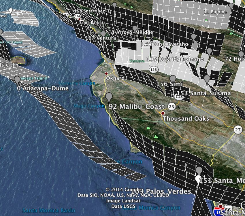
Overview

• Introduction
• The Computational Infrastructure for
  Geodynamics
• Virtual Quake
• Research Code Development Guidelines

4/10/15                                  2
My Background
• University of California, Berkeley 2002
• Ph.D. Computer Science, Osaka University, 2010
• Postdocs at UCDavis, INRIA Grenoble Rhone-Alpes
• My research orientation is scientific computation with a
  computer science focus
• Past projects include work in radio and optical astronomy,
  symbolic mathematics, evolutionary algorithms, large scale
  computing systems, biophysics simulations, supercomputer
  system analysis, geophysics simulation
• Until recently, worked at Computational Infrastructure for
  Geodynamics (CIG) at UCDavis

4/10/15                                             3
CIG
• Computational Infrastructure for Geodynamics
• NSF funded research center
• CIG I – started in 2005 at California Institute of Technology
• CIG II – moved to the University of California, Davis in 2010
• CIG III – scheduled to start in 2015 at UCDavis
• 72 member institutions and international affiliates around
  the world
• Goal is to “[advance] earth science by developing and
  disseminating software for geophysics and related fields”
• CIG provides training for earth scientists, organizes
  workshops, develops research code
• Homepage is at http://geodynamics.org/

4/10/15                                                4
CIG
• Why rewrite geophysics codes that have been already written?
  Don’t!
• “If I have seen further it is by standing on the shoulders of giants.” –
  Isaac Newton
• CIG supports researchers and scientists to share and reuse
  geophysics scientific code
• Covers a wide range of solid earth disciplines including seismology,
  short term tectonics, long term crustal deformation, mantle
  convection, geodynamo
• I’ll briefly discuss some codes that may be useful to your research
• All these and more are available at geodynamics.org/cig/software/

4/10/15                                                          5
SPECFEM
• Numerical modeling of seismic
  wave propagation using spectral
  elements
• Multiple variants, including
  SPECFEM1D, SPECFEM2D,
  SPECFEM3D Cartesian,
  SPECFEM3D Globe
• Specify a source mechanism and
  topography, then determine ground
  acceleration and shaking at different locations
• Used for seismic tomography inversions

4/10/15                                       6
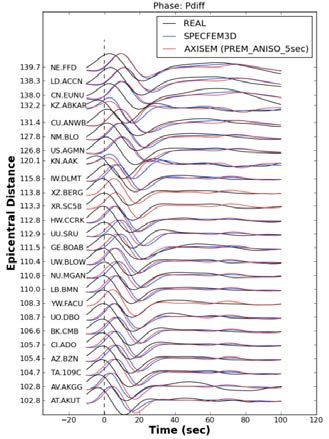
SPECFEM
• Simulate seismic wave
  propagation through
  hypothetical model
• Compare synthetic
  seismograms with actual
  seismograms
                                       Initial mantle tomography
• Update mantle/crust material        (left) and iteratively refined
  model accordingly                        tomography (right)
• Allows for high resolution imaging of whole earth
  structure
• Huge computational cost (10^3 or more core-years)

4/10/15                                                     7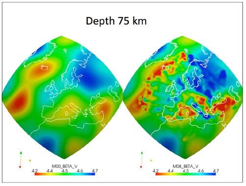
SPECFEM

• Example visualization of SPECFEM3D
  simulation of 1964 Alaska M9.2 earthquake

4/10/15                                 8
SW4
• Seismic wave propagation
  modeling with arbitrary 3D
  heterogeneous material
• User specified source function
• Free surface condition on top
  boundary (allows arbitrary
  topography)
• Developed at Lawrence Livermore National
  Laboratory
• Used for ground motion prediction
• Available at geodynamics.org/cig/software/sw4/

4/10/15                                    9
AxiSEM
• Spectral element method for 3D (an-
  )elastic, anisotropic and acoustic wave
  propagation in spherical domains
• Uses 2.5D approach for fast computation
  – spherical shell layers are assumed
  homogeneous
• Uses series of multipoles to calculate
  response to point source
• Generate synthetic seismograms from
  source functions propagated through
  whole globe at high frequencies
• Available at
  geodynamics.org/cig/software/axisem/

4/10/15                                     10
PyLith
 • Finite element code for dynamic and
   quasistatic simulations of crustal
   deformation, primarily earthquakes
   and volcanoes
 • Primarily used to do highly detailed
   study of stress buildup and rupture
   process of a single fault
       – Strain accumulation associated with
         interseismic deformation
       – Coseismic stress change and fault slip
       – Postseismic relaxation of the crust
 • Available at geodynamics.org/cig/software/pylith/
 4/10/15                                          11
Virtual Quake • Virtual Quake (VQ) is a boundary element code that performs simulations of fault systems based on stress interactions between fault elements • Allows statistical study of fault system behavior and interaction • Over 100 downloads of the software from dozens of countries • Freely available at geodynamics.org/cig/software/vq 4/10/15 12
Overview

• Introduction
• The Computational Infrastructure for
  Geodynamics
• Virtual Quake
• Research Code Development Guidelines

4/10/15                                  13
Virtual Quake
 • First version written by Prof. John Rundle in 1988
       – Could only model small strike slip fault systems
 • Updated in early to mid-2000s by Yakovlev to
   include major strike-slip faults in California and
   named “Virtual California”
 • In 2010 rewritten by Heien to allow parallel
   simulation, arbitrary fault systems
 • Advanced tools for visualization and analysis
   written in 2011-2013
 • Renamed “Virtual Quake” and publicly released
   in 2014

 4/10/15                                                14
Virtual Quake
• Ensemble-domain vs. time-domain simulations
• Time-domain: Understand system behavior by
time stepping through single system
– Generally finite element, or finite difference
– Examples: SPECFEM, AxiSEM, PyLith
– Pros: based on PDE rules, can confirm results
compared to analytical solutions
– Cons: very sensitive to initial conditions, very sensitive
to model configuration, expensive to calculate
(months or years of computer time)
4/10/15 15Virtual Quake
• Ensemble-domain: Understand system behavior in a
statistical manner by studying multiple systems
– Examples: Virtual Quake, climate simulations
– Pros: less sensitive to initial conditions or system
configuration, can be less expensive to calculate (hours or
days of computer time)
– Cons: difficult to exactly compare with mathematical or
experimental models
• We don’t know the current stress state of the faults
– Run an ensemble of simulations to determine which paths
(series of earthquake events) are most likely
4/10/15 16Virtual Quake
• In VQ the earthquake cycle is divided into two parts
– Long term stress accumulation (slider block model)
– Rapid release of stress during rupture
• Long term stress accumulation
– Displacements of faults in the crust
generate stress in surrounding areas
– Displacement is modeled by
movement of fault patches at a
specified constant rate (long term
slip rate)
– Fault patches do not actually
move over time, but rather slip Courtesy (Bak, 1996)
back to their original position during
a rupture event
4/10/15 17Virtual Quake
• Release of stress during rupture
– Fault element failure (rupture) is determined by
Coulomb failure function (CFF)
– Faults can experience either static or dynamic failure
– Static failure: normal stress
is overcome by shear stress
and fault fails (CFF > 0)
– Dynamic failure: change in
stress during a rupture is high
enough that element fails
while CFF < 0
– Rupture occurs in multiple
steps, or “sweeps” (shown right)
4/10/15 18Virtual Quake
• Simulation flow
– Stress accumulation in blue
– Rupture propagation in purple
4/10/15 19Virtual Quake
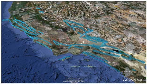
• Fault System Mesher
– Before running a simulation, fault geometry must be
specified
– Define points along fault traces and specify fault
parameters at each point
(depth, rake, dip, etc)
– The mesher creates a set of
elements corresponding to
the faults with the specified
parameters
– The simulation uses this
mesh to calculate stress
interaction and rupture
California fault system meshed
mechanics with 3km x 3km elements
4/10/15 20Virtual Quake
• Mesher supports:
– Input from fault traces (CA faults
included with VC), EQSim format
– Output to ASCII, HDF5, KML
– Mixing elements of different
resolution
– Simple addition/removal of faults
– Merging duplicate vertices to
reduce space, clarify fault element
connectivity
– Automatic stress/friction calculation HDF5 CA Model File
appropriate to model
4/10/15 21Virtual Quake
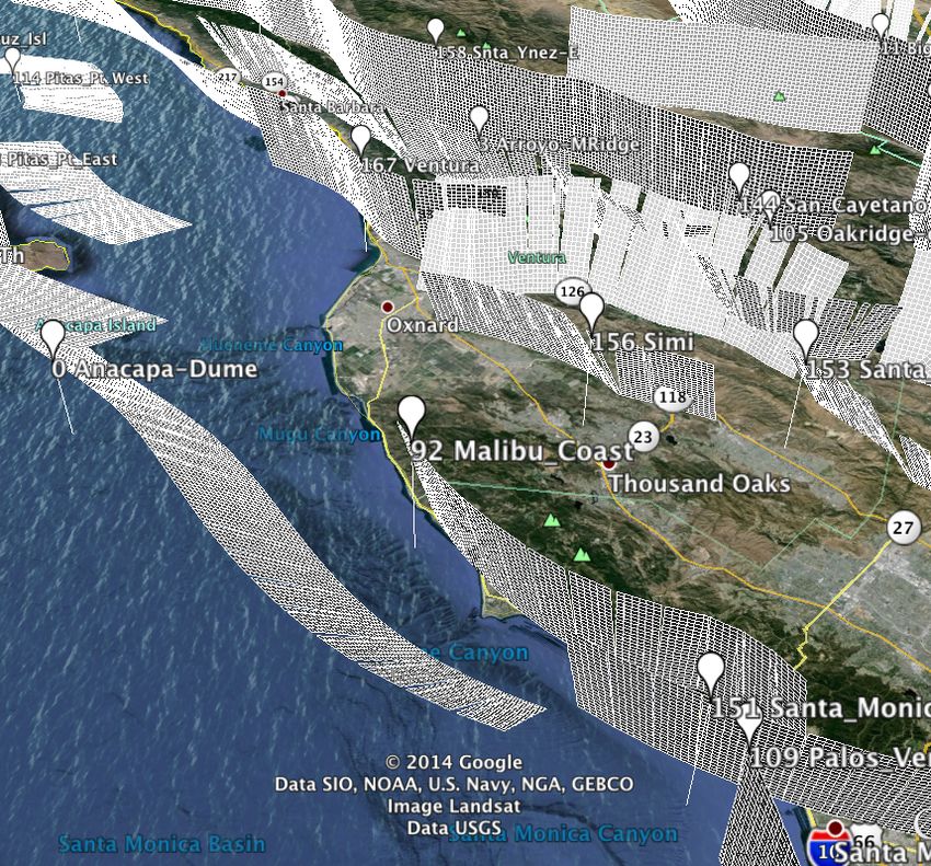
Southern CA faults meshed at 3km resolution (left) and 500m resolution (right)
4/10/15 22Virtual Quake
• Long term stress accumulation
– Interaction between fault elements
is modeled by Okada
implementation[1] of stress transfer
Greens function
Strike slip fault stress
– Functions relate point or field (top view)
rectangular patch displacement to
surrounding a) displacement field,
b) stress field, c) gravity changes
– Interactions between N elements is
stored as an NxN matrix Strike-slip fault stress
[1] Internal Deformation Due to Shear and Tensile Faults in a Half-Space, Y. Okada 1992 field (side view)
4/10/15 23Virtual Quake
• Long term stress accumulation
– Calculate stress interaction between all elements
and store in a matrix where TAB is the stress
change on A caused by B moving a unit distance
– Buildup of stress on element A is determined by
– or in the matrix notation
– This is equivalent to a matrix-vector multiply
4/10/15 24Virtual Quake
• Initial fault element failure
– VQ uses the CFF (Coulomb Failure Function) to
determine when an element fails
– VQ treats normal stress as constant and shear stress
as increasing, so eventually a fault will fail due to the
CFF criteria
• Can have variable normal stress for thrust faults
– An element fails when CFF > 0, which means shear
stress overrides normal stress and friction
4/10/15 25Virtual Quake
• Rupture propagation
– For a failed element, initial slip is determined by the
relation
where KL is the self-shear stress of the element
– In previous versions of VQ (and most other similar
codes), element slip was prescribed in the model by
modifying the stress drop (Δσ)
– This allowed the user to force faults to have arbitrary
magnitude earthquakes
– In the current version of VQ, initial slip is determined
mathematically to ensure faults obey scaling laws
4/10/15 26Virtual Quake
• Rupture propagation
– After elements have been processed, we determine if
more elements will fail
– Elements can rupture due to static failure (CFF>0) or
dynamic failure
– Dynamic failure occurs if
and corresponds to how likely the crack tip will
propagate
– The value of η determines how much a rupture will
grow (small η means larger earthquakes)
4/10/15 27Virtual Quake
• Rupture propagation
– We have tried using rate state friction based on the standard
formulation
– This is an advanced friction model that allows for fault healing and
slow stress buildup
– Nondimensional version on the
equations is shown to the right
– For a single block within a
range of parameters this works
as a good model
– However, because of the ln(V) and
ln(Θ) terms in the force, V and Θ must not become negative
– With coupled block systems you cannot guarantee these will not be
negative because of the interaction with other blocks
– Most “rate-state” simulators use a simplified form of these equations
4/10/15 28Virtual Quake
• The parameter η must be tuned to
best match actual magnitude-
frequency distributions
• In our experience, η=0.4 to 0.8 is
generally best
• Plots on the right show how well
frequency magnitude corresponds
to common models
– Top is UCERF2 observed seismicity
– Bottom is Wells and Coppersmith
relation
• Within the η=0.5 to 0.7 range we
get good fit to observed seismicity
4/10/15 29Virtual Quake • By running a long simulation and analyzing the event catalog, we can make forecasts about interval times • Figure on the right shows the conditional cumulative probability of a M≥7.0 earthquake on forecasted faults (Northern CA) • Based on event catalog from VQ simulation covering thousands of years (multiple event cycles) • Distribution is evaluated at t=t0+Δt with the last earthquake occurring t0 years ago 4/10/15 30
Virtual Quake
 • Forecast waiting times
   for next M≥7.0
   earthquake on northern
   CA faults
 • Dark line is median waiting
   time (50% probability)
 • Yellow band is 25-75%
   probability band
 • The dashed vertical line indicates elapsed time since
   last M≥7.0 (Loma Prieta 1989)
 • Based on this, 25% probability of M≥7.0 in northern CA
   within ~5 years

 4/10/15                                          31
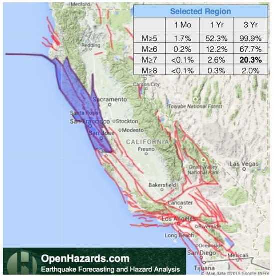
Virtual Quake
• VQ comparison to other
forecasts
• OpenHazards.com
– Provides free
magnitude/time estimates
for arbitrary regions
– Operated by Prof. John
Rundle
• Estimate of M≥7 over next
3 years is 20.3%
• VQ prediction of M≥7 in
same area is 14.7%
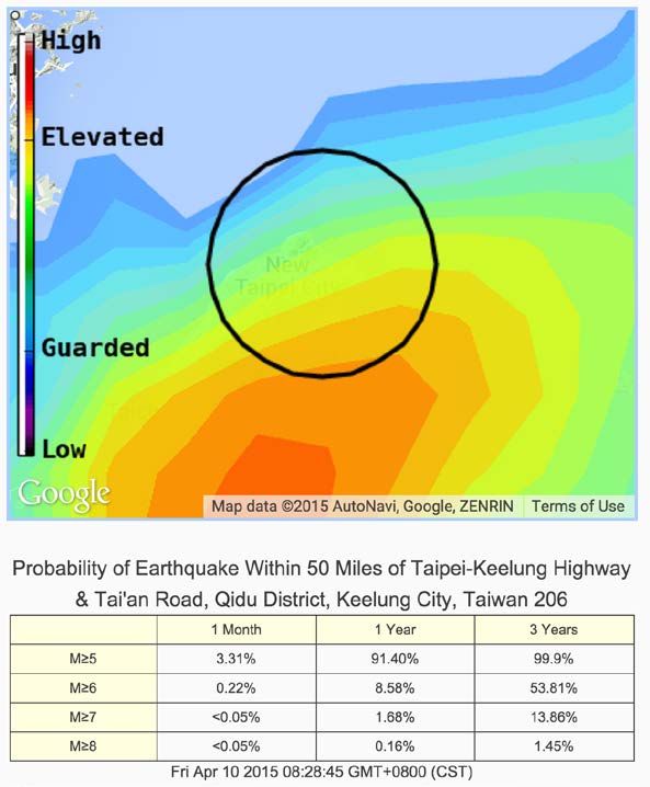
4/10/15 32Virtual Quake • Estimate for Taipei area (as of this morning) • M≥5 in 1 year, 91% probability • M≥7 in 1 year, only 1.7% probability • Conditional Weibull method of forecasting (counting earthquakes) 4/10/15 33
QuakeLib/PyVQ

• VQ usage involves the following steps:
      – Create 1D model of fault system based on traces
      – Run trace model through mesher to generate 3D
        model of fault system
      – Define simulation parameters (simulation length,
        dynamic rupture propagation parameter, etc)
      – Run simulation(s)
          • Read model file
          • Calculate Greens function
          • Output data files from simulation
      – Analyze output files, generate visualization

4/10/15                                                34
QuakeLib/PyVQ
• Most of these steps have computational steps in
common
– Read and write files with the fault model and event
history
– Vector mathematics
– Manipulating and querying fault representations
– Stress, displacement, gravity anomaly calculations
(based on Greens functions)
• Rather than implementing the same functionality
multiple times, VQ uses QuakeLib
• QuakeLib provides access to shared functionality
through a C, Python, or other interface
4/10/15 35QuakeLib/PyVQ • Once data is generated from the simulation, tools are needed to analyze and visualize results • PyVQ is a Python based toolkit built on QuakeLib • Provides functionality to plot events on maps, magnitude- frequency/cumulative distributions, analyze interevent times, fault interconnectivity • Right graphic shows a visualization of InSAR interferogram fringes of multiple events from a VQ run 4/10/15 36
QuakeLib/PyVQ
• PyVQ also calculates gravity changes from displacement of a fault
  patch
• This will be correlated with NASA GRACE (Gravity Recovery and
  Climate Experiment) mission data to evaluate gravity changes as a
  means of detecting faults
• Figure below shows the surface gravitational anomalies for a strike
  slip fault (left), normal fault (center), and thrust fault (right)
• Gravity anomaly calculations based on Okubo[2]

[1] Gravity and potential changes due to shear and tensile faults in a half-space., S. Okubo 1992

4/10/15                                                                                             37
GPGPU Support
• Working with Optimal
  Synthesis we implemented
  GPU (CUDA) based support
  for VQ calculations
• Focused on two compute intensive sections of code
      – Green’s function calculation (N^2 calculations, each
        requiring 14,000-45,000 flops)
      – Long term stress calculate (N^2 flops between each event,
        1e5-1e7 events per simulation)
      Model Name        Elements (N)   Matrix Size   CPU Times (12-Core)
AllCal2_Trunc7453          7453        423.96 MB      371.49s (6m 12s)
AllCal2_NoCreep_13482      13482        1.35 GB      5137.03s (1h 25m)
AllCal_17757               17757        2.35 GB      3432.16s (57m 12s)

4/10/15                                                                    38
GPGPU Support
• Results on GPU are highly promising
• Green’s function calculation is 80x
faster than single CPU core,
7.3x faster than 12 cores
– Branching rarely affects Green’s NVIDIA
Titan
function in normal fault configurations
• Matrix-vector multiply (stress accumulation
phase) is 45x faster than single core, 47x faster
than 12 cores (memory bandwidth limited)
• Total simulation runtime is 32-50x faster on GPU
4/10/15 39GPGPU Support (graph courtesy Optimal Synthesis) 4/10/15 40
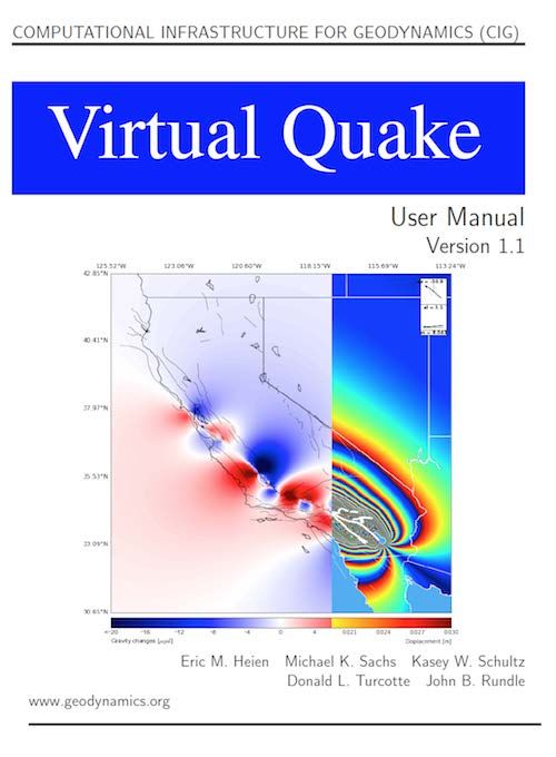
Virtual Quake
 • Current version is available at
       – geodynamics.org/cig/software/vq
 • Includes
       – Improved mesher
       – Example files, introductory tutorial
       – Manual describing code background,
         physics equations, and input/output
         file formats
       – QuakeLib and Python wrappers used for PyVQ and
         WebVC visualization/analysis
       – 235 unit tests covering all aspects of the code
       – Parallel calculation with OpenMP and MPI

 4/10/15                                            41
Virtual Quake
• We want arbitrarily small
elements so we can properly
model small magnitude
earthquakes
• 3000m x 3000m elements
result in minimum magnitude
of around M=5.6
• Memory and speed are significant limitations
– Interaction matrix size grows as N^2 in elements
– Elements grow as N^2 in resolution
– Therefore, memory requirements grow as N^4
• Example: for CA fault system, 3000m resolution requires ~1GB of
memory, 500m resolution requires ~5000GB of memory
4/10/15 42Future Development
• Currently limitation to detailed simulations is memory
usage
– Grows as O(N^4) – CA model at 250m
resolution (2 million elements) would
require 30 TB memory
– Hierarchical matrix implementation
reduces this to O(N^2) – (e.g. 32GB for
2 million elements)
– Also significantly improves runtime Sample Hierarchical Matrix
• Dynamic fault geometry
– Current fault configuration is static – what happens when faults
change over time?
• Improve analysis/visualization tools (PyVQ, WebVQ)
– Simplify analysis for users, provide web frontend
4/10/15 43Overview • Introduction • The Computational Infrastructure for Geodynamics • Virtual Quake • Research Code Development Guidelines 4/10/15 44
Research Code Guidelines

 • My background is in computer science
 • There are several practices common in
   computer science that benefit research code
   development
       – Version control
       – Unit testing
       – Continuous integration
       – Use libraries/modules
 • Using these tools will make your research
   more efficient, accurate, and reproducible
 4/10/15                                   45
Research Code Guidelines
• Version control
– Code changes over time
– Very useful to track what was changed when
– Version control keeps a record of what was changed for what
reason at what date
– Helps ensure reproducibility, keeps a record of who changed
what at what time
– Allows multiple researchers to collaborate on the same project
simultaneously
– I recommend Git and
Github (try.github.io)
– Makes it easy to share
your code with others –
Git development history for VQ
becoming a requirement
for many journals
4/10/15 46Research Code Guidelines
• Continually add tests to confirm code validity
• Virtual Quake:
– 235 tests run automatically after each code change
– Tests are run on multiple platforms to find platform
dependent problems
– Confirm basic mathematical and vector operations
function correctly
– Verify that simulations produce expected results
– Verify that multiple processors yield same results as single
processor
– Confirm Green’s function calculation produces results
within expected tolerances
– Confirm file reading/writing function as expected
4/10/15 47Research Code Guidelines
• Libraries
– Much of the functionality you need for your research
has already been written
– Finite element: deal.II, PETSc, Fenix
– Linear algebra: Trilinos, PETSc, LAPACK
– Data analysis and visualization: matplotlib, scipy,
numpy
– Earthquake/Seismic: ObsPy, QuakeLib, OpenSHA
• Research is an iterative process
– Automate as much as possible
– If you are typing the same thing over and over, or
copying/pasting data, you are wasting your time
4/10/15 48Conclusion • Virtual Quake is a boundary element code to simulate long term fault stress interactions for statistical study • Uses Greens functions for stress interaction between faults, static/dynamic failure model for rupture propagation • Results with California model show good agreement with observed seismicity • Provides a means to do event recurrence forecasting • Provides tools for analysis and visualization of data 4/10/15 49
Thank you

Any questions?
You can also read