Numerical Weather Models for Tropospheric Mitigation in Marine Kinematic GPS: a Daylong Analysis
←
→
Page content transcription
If your browser does not render page correctly, please read the page content below
Numerical Weather Models for Tropospheric
Mitigation in Marine Kinematic GPS: a Daylong
                   Analysis
                                               Felipe G. Nievinski
                Department of Geodesy and Geomatics Engineering, University of New Brunswick, Canada

BIOGRAPHY                                                     INTRODUCTION

Felipe Nievinski is a M.Sc.E. student and research            GPS radio signals are refracted when they propagate
assistant at the Dept. of Geodesy and Geomatics               through the Earth's neutral atmosphere (the bulk of which
Engineering, University of New Brunswick. At the end of       is the troposphere but also includes the stratosphere).
2004 he received his degree in Geomatics Engineering          Timing (ranging) of GPS signals is delayed (increased)
from the Federal University of Rio Grande do Sul, Brazil.     compared to what would be measured if the signals
He is a member of the Institute of Navigation, the            propagated in a vacuum. In other words, the distance
American Geophysical Union, and the Society for               measured with GPS signals propagating through the
Industrial and Applied Mathematics.                           neutral atmosphere is always greater than the geometrical
                                                              distance between satellite's and receiver's antennas. The
ABSTRACT                                                      delays (hereafter tropospheric delays) range from 2.3 m at
                                                              zenith to approximately 26 m at 5º elevation-angle, for a
It has been recommended that, “in precise [static]            station on the geoid [Seeber, 2003].
applications where millimetre accuracy is desired, the
delay must be estimated with the other geodetic quantities    It has been recommended that, “in precise [static]
of interest” [McCarthy and Petit, 2004, p. 100]. While        applications where millimetre accuracy is desired, the
that recommendation is common practice in static              delay must be estimated with the other geodetic quantities
positioning, tropospheric delay remains as one of the         of interest” [McCarthy and Petit, 2004, p. 100]. While
main error sources in medium to long-distance kinematic       that recommendation is common practice in static
positioning. Its mitigation is more challenging in            positioning, tropospheric delay remains as one of the
kinematic applications because its strong correlation with    main error sources in medium to long-distance kinematic
the vertical coordinate is aggravated by the need to          positioning. Its mitigation is more challenging in
estimate the rover position at every epoch.                   kinematic applications because its strong correlation with
                                                              the vertical coordinate is aggravated by the need to
In this paper we report one further step in our               estimate the rover position at every epoch.
investigation on the use of Numerical Weather Models
(NWM) for predicting tropospheric delays, aiming at           Whereas some authors recommend that the simultaneous
improvements in kinematic applications. We analyze a          estimation of position and tropospheric parameters be
daylong session. Our results show that NWM yields a           avoided [Schüler, 2006], others have tried to overcome
slight improvement in height bias, with no improvement        this limitation [Dodson et al., 2001]. Both approaches
in horizontal bias. Observation residuals show no             would benefit from more realistic initial values for the
significant change.                                           troposphere, such as the ones given by Numerical
                                                              Weather Models (hereafter NWM) [Cucurull et al., 2002].
We have shown that NWM have only marginal
improvement on a 70 km kinematic baseline over well-          NWM are generated by “the integration of the governing
established, simpler, tropospheric delay prediction models    equations of hydrodynamics by numerical methods
(Saastamoinen, UNB3m). As ray-tracing in NWM is far           subject to specified initial conditions” [Glickman, 2000].
more complex and computationally more expensive than          Global and regional NWP models are produced daily by
those simpler models, they should be preferred until one      several meteorological agencies throughout the world,
demonstrates that the impact in using NWM tropospheric        mainly for weather forecasting purposes.
delay predictions is, indeed, far superior.
In addition, the marine environment poses unique
challenges, due to, e.g., rapid-varying weather conditions
and large gradients in pressure, temperature, and humidity
from mainland to sea.
In this paper we report one further step in our
investigation on the use of Numerical Weather Models for
predicting tropospheric delays, aiming at improvements in
kinematic applications. In the past, only 1 h [Nievinski et
al., 2005; Ahn et al., 2006, Cucurull et al., 2002], 5 h
Figure 1: Ferry boat employed as rover station.
[Cove et al., 2004], and 6 h [Jensen, 2002] kinematic
sessions were analyzed; we speculate that is due to the
large amounts of data that comprises NWM. In this paper
we analyze a daylong session.
Our paper is organized as follows. First we describe the
data used and the methods employed. Second we show
and discuss the results obtained. The paper finishes with a
summary of our findings.
DATA
We used dual-frequency GPS observations collected at 1
Hz sampling rate, over 1 full day, at 2 base stations and at
one rover station. We downsampled the data to 30 s-1 rate, Figure 2: Map of the base stations.
in order to allow us to experiment with different
processing settings in a timely manner. The rover is
installed on a ferry boat (Figure 1) that goes back and
forth across the Bay of Fundy, South-Eastern Canada,
between the cities of Digby (N.S.) and St. John (N.B.), 75
km apart (Figure 2). The day selected was September 30,
2004, the most recent day for which we have full GPS
data at the 3 stations, collected during the yearlong
Princess of Acadia Project [Santos et al., 2004]. During
that day the ferry crossed the bay 6 times.
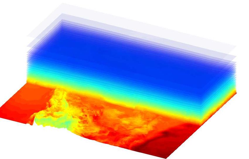
We also used grids from the Canadian Global
Environmental Multiscale Numerical Weather Model
[Côté et al., 1998] (Figure 3). Its resolution is as follows: Figure 3: 3-dimensional refractivity field (unitless), as
15 km nominal (horizontal); 28 variable-height isobaric given by the Northern half of the GEM NWM. Height
levels plus 1 ground level (vertical); 3 h (temporal). The exaggerated 100 times.
NWM is initialized every 0 and 12 h UTC, at which 16 3- 0
hourly grids are issued covering the following 48 h
period. For the full day of September 30, 2004, we used -1000
the following grids (in the format initialization epoch +
forecast intervals): September 30, 0 h +0,+3,+6,+9 h; -2000
Northing (km)
September 30, 12 h +0,+3,+6,+9 h; and October 1st, 0 h
+0 h. -3000
We also used profiles of meteorological data (pressure, -4000
temperature, and relative humidity), collect by
radiosondes launched from 89 sites over all of the NWM -5000
continental extent (Figure 4), at September 30, 0 h UTC.
-2000 -1000 0 1000 2000 3000 4000
Easting (km)
Figure 4: Location of the radiosonde launching sites.METHODS We evaluated two tropospheric delay prediction models in
addition to NWM: UNB3m [Leandro et al., 2006] and
Generation of the NWM tropospheric delay Saastamoinen with standard weather parameters reduced
predictions to the station height. For the multi-base station solution
we employed the Saastamoinen model only. We did not
We employed the ray-tracer described in Nievinski et al. estimate residual tropospheric delay in any kinematic
[2005]. In the past, we have ray-traced directly slant solution.
delays; for this paper, we decided to ray-trace only zenith
delays and map them to lower elevation angles using For PPP processing, we employed the Canadian Spatial
Niell’s mapping function [Niell, 1996]. The motivation Reference System on-line PPP application1. It predicts
for that was to reduce the total ray-tracing processing time zenith tropospheric delay with Saastamoinen model as
– in effect, we reduced it by a factor of 7, the mean used in this paper, and also estimates residual
number of visible satellites. The justification for that tropospheric delay every epoch.
decision is that it is valid to study separately the delay at
zenith and its elevation-angle dependence. Perhaps it is Validation of the NWM tropospheric delay predictions
not only valid but also more useful, since it allows one to
make separate conclusions about the usefulness of NWM To validate the NWM tropospheric delay predictions we
for each aspect. In effect, we have put the study of the compared them to radiosonde predictions. Radiosonde is
second aspect (see, e.g., Böhm and Schuh, 2004) outside often employed as benchmark in the validation of
the scope of this paper. tropospheric delay prediction models (e.g., Mendes,
1999). It gives us hydrostatic and non-hydrostatic partial
Generation of the GPS positioning results delays separately, allowing us to validate each
component.
We had two scenarios: one is the kinematic processing of
a moving rover; another is the kinematic processing of a Validation of the GPS positioning results
stationary rover. In each scenario we had (i) a reference
solution and (ii) test solutions. Solution (i) should be more We validated the GPS positioning results to assure we had
accurate and precise than any of (ii), so as to allow us to reliable reference solutions vis-à-vis their respective test
safely attribute any discrepancy between the two to errors solutions. To do so, we checked the following two
in (ii). statistics: formal standard deviation and forward/reverse
solution separation. Even though usually the reported
In the stationary rover scenario, the test solutions were formal standard deviations are too optimistic, we expect
generated taking one of the base stations as rover. The them to be consistently larger and smaller for worse and
reference solution comes from a weighted average of 5 better solutions, respectively. The forward/reverse
static, precise point positioning daily solutions, spanning separation is the discrepancy between the two solutions
September 27 to October 1st, 2004 (inclusive). given for the same baseline, obtained using exactly the
same data and settings, as a feature of Kalman filters such
The moving rover scenario is more challenging because, as the one employed in GrafNav. Again, it is not exactly a
e.g., cycle slips will be more numerous and more difficult measure of accuracy, but we expect it to be consistently
to detect and fix. The test solutions are the individual larger and smaller for worse and better solutions, so as to
baseline solutions Digby-Ferry and St. John-Ferry. The allow us to use these statistics to draw a conclusion about
reference solution is a multi-base station solution, in the relative quality of reference and test solutions.
which the GPS observations collected at both base
stations and at the Ferry are processed in the same Assessment of the impact of NWM tropospheric delay
Kalman filter. This multi-base station solution is better predictions on the GPS positioning results
than processing each individual baseline separately and
adjusting the ferry positions after the fact. For both moving and stationary rover scenarios, we
assessed the accuracy of the rover test solutions to the
For the GPS kinematic processing, we employed respective reference solutions. We also checked the phase
NovAtel’s (Waypoint Products Group) GrafNav Batch, and code measurement residuals.
version 7.60. We applied a 10º cut-off elevation angle,
and satellites were weighted inversely proportional to the
sine of their elevation angle. The L2 signal was used to
help fix ambiguities. The L2 signal was also used to
correct for ionospheric delay in all but the multi-base
station solution – for discussion, please see section below.
1RESULTS AND DISCUSSION
Validation of the NWM tropospheric delay predictions
We compared NWM delays against radiosonde delays at
the epoch September 30, 2004, 0 h UTC. We found 2
centimetric biases and spread (summarized in Table 1), 0
out of an average total delay amounting to 2.3 m.
-2
Please notice in Figure 5 that the bias and spread in total
30 40 50 60 70 80 90
delay correspond, respectively, to a bias in the hydrostatic
component and to a spread in the non-hydrostatic
component. The bias can be explained by an inaccurate 2
transformation to geopotential heights, as part of the ray-
0
tracing procedure. In the past we have found decimetric
biases for this reason [Nievinski, 2005], which were fixed -2
and reduced to the level presented here. The spread is
expected for the non-hydrostatic delay, function of 30 40 50 60 70 80 90
humidity hence highly variable and harder to predict.
Also notice that the spread decreases towards higher 2
latitudes; again, that is expected, since humidity in the air
decreases towards the pole. 0
-2
To further investigate the bias found in hydrostatic delay,
we compared the NWM ray-traced value to the value 30 40 50 60 70 80 90
obtained using Saastamoinen’s formula and surface Latitude (degrees)
pressure as interpolated in the NWM (we call this NWM
self-discrepancy in hydrostatic delay). Comparison results Figure 5: Discrepancy (in cm) between NWM and
shown in Figure 6 resemble closely the discrepancies radiosonde delays. Top panel: total delay; Center panel:
found in hydrostatic delay between NWM and hydrostatic delay; Bottom panel: non-hydrostatic delay.
radiosonde. That is an ongoing research issue.
Table 1: Statistics (in cm) for discrepancy between NWM
2
and radiosonde delays.
Mean Rms Std 0
Total Delay 1.05 1.29 0.75
Hydrostatic Delay 1.15 1.18 0.25 -2
Non-Hydrostatic Delay -0.1 0.69 0.69
30 40 50 60 70 80 90
Latitude (degrees)
Table 2: Statistics (in cm) for NWM self-discrepancy in
hydrostatic delay. Figure 6: NWM self-discrepancy in hydrostatic delay (in
Mean Rms Std cm).
Hydrostatic Delay 1.24 1.26 0.22Validation of the GPS positioning results – stationary Validation of the GPS positioning results – moving
rover scenario rover scenario
The reference solution in the stationary rover scenario First we inspected the forward/reverse separation and also
provides coordinates with milimetric repeatability and the formal standard deviations (Table 6 and Table 7).
sub-milimetric formal standard deviations (Table 3),
which we consider too optimistic. A more realistic figure
Table 6: Rms (in cm) of forward/reverse separation.
is given by Kouba [2003], who demonstrates that with
(Leftmost column indicates base station).
PPP and IGS products one can estimate station
coordinates with centimetric accuracy. Height Latitude Longitude
Table 3: Base station coordinates. no model 19.3 13.9 8.7
St. Saastamoinen 14.8 7.3 6.3
Height Latitude Longitude John UNB3m 11.6 5.6 7.2
Digby 37.4462 44º 37' -65º 45' NWM 15.6 5.9 5.4
m 13.790254" 34.9665" no model 33.9 15.8 20.9
(std) 2.0 mm 0.4 mm 0.9 mm Saastamoinen 6.5 3.9 3.7
St. John 4.5362 m 45º 16' -66º 03' Digby
UNB3m 6.6 3.4 5.0
17.54366" 46.686244" NWM 6.4 3.4 4.7
(std) 2.0 mm 0.6 mm 1.2 mm Multi-base station 7.3 4.4 4.5
We inspected the statistics for the test solutions (Table 4
and Table 5). We give statistics only for the baseline with Table 7: Formal standard deviations (in cm). (Leftmost
Digby as base and St. John as rover because the second column indicates base station).
baseline (with exchanged base and rover) has values with Height Latitude Longitude
nearly identical magnitude and biases with reversed sign. no model 7.3 4.0 2.8
Since those figures are all larger than 1 cm, we concluded
St. Saastamoinen 7.3 4.0 2.8
that the PPP solution can be used as a reliable reference in
John UNB3m 6.7 3.7 2.6
the stationary rover scenario.
NWM 6.6 3.7 2.6
Table 4: Rms (in cm) of forward/reverse separation; no model 6.4 3.6 2.7
baseline with Digby as base and St. John as rover. Saastamoinen 6.5 3.6 2.7
Digby
Height Latitude Longitude UNB3m 6.0 3.3 2.4
no model 51.8 21.1 26.4 NWM 6.4 3.3 2.4
Saastamoinen 9.6 6.6 5.7 Multi-base station 3.6 2.1 1.5
UNB3m 6.9 3.7 3.7
NWM 7.0 3.8 3.8 The overall statistics are consistently better for the
reference, multi-base solution, than for any of the test
Table 5: Formal standard deviations (in cm); baseline solutions. Yet, a closer inspection at the time series of
with Digby as base and St. John as rover. those discrepancies reveals that, even though the multi-
base station solution is almost always better than the
Height Latitude Longitude
individual baseline solutions, during certain periods it is
no model 8.4 4.8 4.0
not significantly better, as required for a reliable
Saastamoinen 8.0 4.4 3.1
reference. For instance, Figure 7 shows that the height
UNB3m 7.0 3.9 2.7
formal standard deviation for the multi-base station
NWM 7.0 3.9 2.7
solution approaches that of NWM-corrected baseline
solutions during certain periods.In addition to an upper distance threshold applied to the
Multi-base reference solution, we applied a lower distance threshold
St. John--Fery baseline to the test solutions. The later is needed because we do
Digby--Ferry baseline
not expect much different impact of different prediction
Ellipsoidal Height Formal Std. (m)
models on short test baselines. As the Ferry goes back and
0.1 forth between Digby and St. John, their respective
individual baselines get shorter and longer, and the
across-receiver observation differencing technique gets
more and less effective in cancelling out the tropospheric
0.05 delay common at both base and rover stations. While the
length of a test baseline is smaller than a given threshold
(baseline height offset being negligible), there is not much
relative, residual, tropospheric delay left for the prediction
models to correct for. Empirically we set that threshold
0
0 6 12 18 24 value to 40 km.
Time (hour of the day, GPST)
To summarize, the combined criteria for meaningful
Figure 7: Time series of rover height formal standard
discrepancies is that the distance to the nearest base
deviation yielded by multi-base station and NWM-
station in the reference solution be smaller than 20 km,
corrected individual baseline solutions.
and the distance to the base station in the test solution be
larger than 40 km. Figure 9 depicts that criteria
Those periods can be defined based on the distance of the graphically (contrast it with Figure 8, top and center
Ferry to the nearest base station (Figure 8). As expected, panels). Please note we are intentionally discarding the
the closer the Ferry is to any base station, the better the epochs at which one could not draw conclusions about the
multi-base station solution will be. Whenever that impact of different tropospheric prediction models.
distance exceeds a certain threshold, the multi-base
Distance to (nearest) base station (km)
station solution, even though better, can no longer be 80
relied upon as a reference solution for the individual
baseline solutions. Empirically we have set that threshold 60
value to 20 km.
St. John
80 40 Digby
60 Multi-base station
St. John
40 20
Digby
20
0
0 6 12 18 24 0
0 6 12 18 24
80
60
Figure 9: periods of each solution for which we can draw
40
conclusions about the impact of different tropospheric
20
prediction models.
0
0 6 12 18 24
0.08
Figure 9 also helps us explain why we decided to use L2
0.06
for ionospheric correction in the test solutions only, but
0.04
not in the reference solution. The increased-noise
0.02
ionospheric delay-free observable is beneficial for the
0 individual long-baseline solutions, but would be
0 6 12 18 24
Time (hour of the day, GPST) unnecessary and even harmful in our multi-base station
solution.
Figure 8: Top panel: distance from Ferry to either base
station (in km); Center panel: distance from Ferry to
nearest base station (in km); Bottom panel: height formal
standard deviation for the multi-base station solution (m).Impact assessment – stationary rover scenario
As in for its validation, we show results only for the
baseline with Digby as base and St. John as rover. The Table 8: Rms of observation residuals (in m); stationary
corresponding figures would be flipped around the zeros rover scenario.
axes.
C/A Code L1 Phase
NWM yields an improvement in height bias, with no no model 0.72 0.037
improvement in horizontal bias. Scattering in longitude is Saastamoinen 0.71 0.018
slightly improved as well. Observation residuals UNB3m 0.74 0.020
surprisingly show no significant change, even when we NWM 0.74 0.020
use no tropospheric model.
Table 9: Statistics for discrepancy (in cm) between test and reference solutions; stationary rover scenario.
Height Latitude Longitude
mean rms std mean rms std mean rms std
no model -7.8 25.2 23.9 8.2 13.7 11 2.6 17.2 17.0
Saastamoinen -2.6 6.7 6.2 0.2 3.7 3.7 1.2 4.1 4.0
UNB3m -2.5 6.0 5.4 0.2 3.2 3.2 1.2 2.7 2.4
NWM -0.9 5.0 4.9 0.0 3.2 3.2 1.1 2.5 2.3
0.15
0.25
Saastamoinen
0.2 UNB3m 0.1
NWM
0.15
Discrepancy in Ellipsoidal Height (m)
Discrepancy in Latitude (m)
0.1 0.05
0.05
0
0
-0.05
-0.05
-0.1
-0.15
-0.1 Saastamoinen
-0.2
UNB3m
-0.25 NWM
0 6 12 18 24
Time (hour of the day, GPST) -0.1 -0.05 0 0.05 0.1 0.15
Discrepancy in Longitude (m)
Figure 10: Time series of discrepancy in height; stationary
rover scenario. Figure 11: Horizontal discrepancy; stationary rover scenario.Impact assessment – moving rover scenario
Table 10: Rms of observation residuals (in m); moving
rover scenario.
Overall, NWM improves the baseline St. John–Ferry C/A L1
(Tables 10 and 11, Figures 12 and 13), both in bias and Code Phase
rms for all coordinates. As for the baseline Digby—Ferry no model 1.23 0.026
(Tables 10 and 11, Figures 14 and 15), NWM only Saastamoinen 1.22 0.020
marginally improves the statistics, with a worsening in St. John
UNB3m 1.22 0.022
height compared to UNB3m. Again, the observation NWM 1.23 0.021
residuals surprisingly show no significant change, even no model 1.07 0.031
when we use no tropospheric model. Saastamoinen 1.05 0.016
Digby
UNB3m 1.05 0.018
NWM 1.05 0.018
Table 11: Statistics (in cm) for discrepancy between test and reference solutions, moving rover scenario.
Height Latitude Longitude
mean rms std mean rms std mean rms std
no model 10.2 16.1 12.5 -8.1 10.2 6.2 -0.8 6.4 6.3
Saastamoinen 2.4 10.5 10.2 -1.6 5.2 4.9 -2.8 5.1 4.3
St. John
UNB3m 4.3 8.0 6.8 -1.9 4.8 4.4 -1.3 3.1 2.8
NWM 1.5 5.8 5.6 -0.9 3.3 3.2 -0.8 2.8 2.6
no model 10.0 21.5 19.1 4.9 11.7 10.6 -5.6 11 9.4
Saastamoinen -1.9 5.9 5.5 0.3 4.1 4.1 1.0 2.3 2.0
Digby
UNB3m -0.5 8.4 8.4 -0.8 4.6 4.5 -1.5 4.0 3.7
NWM 0.9 9.2 9.1 -0.6 4.3 4.2 -1.5 3.8 3.5
CONCLUSION Our aim is to determine the baseline length for which
NWM tropospheric delay starts to be far superior to well-
We have shown that NWM have only marginal established, simpler tropospheric delay prediction models.
improvement on a specific 70 km kinematic baseline over
well-established tropospheric delay prediction models As a long-term goal, we would like to extend the analysis
(Saastamoinen, UNB3m). As ray-tracing in NWM is far presented in this paper to yearlong sessions, so as to cover
more complex and computationally more expensive than different seasons and anomalous atmospheric conditions.
those simpler models, they should be preferred until one
demonstrates that the impact of NWM tropospheric delay ACKNOWLEDGMENTS
predictions is, indeed, far superior.
- Prof. Dr. Marcelo Santos, University of New Brunswick,
ONGOING AND FUTURE WORK for supervision;
- Mr. Rodrigo Leandro, University of New Brunswick, for
To introduce the predicted delays, currently we are (i) fruitful discussions and also for providing the PPP
converting the receiver-specific observation files to solution and radiosonde ray-traces;
RINEX and then (ii) subtracting the predicted delays from - NOAA for the radiosonde data;
the raw observations, yielding corrected RINEX - Canadian Meteorological Centre for the NWM;
observation files. We are aware that this approach is not - Geodetic Survey Division of NRCan for their PPP
the best, in the sense that in (i) we may lose information application;
about cycle slips already detected by the receiver itself, - Canadian International Development Agency (CIDA)
and in (ii) we may be introducing additional cycle slips. for funding;
Therefore we are working to be able to introduce the - Office of Naval Research, through University of
predicted delays at the estimation level. Southern Mississippi, and National Science and
Engineering Research Council (NSERC), for financial
As future work, we plan to process a number of varying- support for the Princess of Acadia Project.
length baselines (from, e.g., 50 up to 1,000 km). These This research is inserted into GEOIDE Project “Next-
will be stationary rovers processed in kinematic mode, so Generation Algorithms for Next-generation algorithms for
as to allow us to assess their accuracy by comparing the navigation, geodesy and earth sciences under modernized
rover position solutions to their known static solutions. Global Navigation Satellite Systems.”0.2
Saastamoinen
0.3 0.15 UNB3m
NWM
Discrepancy in Ellipsoidal Height (m)
Discrepancy in Latitude (m)
0.2 0.1
0.05
0.1
0
0
-0.05
-0.1
-0.1
S aas tam oinen
-0.2 UNB 3m
-0.15
NW M
-0.2
0 6 12 18 24 -0.2 -0.1 0 0.1 0.2
Tim e (hour of the day , G P S T) Discrepancy in Longitude (m)
Figure 12: Time series of discrepancy in height; moving Figure 13: Horizontal discrepancy; moving rover scenario,
rover scenario, baseline St. John – Ferry. baseline St. John – Ferry.
0.2
Saastamoinen
0.15 UNB3m
NWM
0.3
Discrepancy in Latitude (m)
0.1
Discrepancy in Ellipsoidal Height (m)
0.2
0.05
0.1
0
0 -0.05
-0.1 -0.1
S aas tam oinen -0.15
-0.2
UNB 3m
NW M
-0.2
0 6 12 18 24
-0.2 -0.1 0 0.1 0.2
Tim e (hour of the day , G P S T) Discrepancy in Longitude (m)
Figure 14: Time series of discrepancy in height; moving Figure 15: Horizontal discrepancy; moving rover scenario,
rover scenario, baseline Digby – Ferry. baseline Digby – Ferry.
REFERENCES GNSS-2004, 21-24 September, 2004, Long Beach, CA,
USA, pp. 925-932.
Ahn, Y. W., G. Lachapelle, S. Skone, S. Gutman, and S.
Sahm. Analysis of GPS RTK performance using external Côté, J., S. Gravel, A. Méthot, A. Patoine, M. Roch, A.
NOAA tropospheric corrections integrated with a multiple Staniforth (1998). The Operational CMC–MRB Global
reference station approach. GPS Solutions, 10 (3): 171- Environmental Multiscale (GEM) Model. Part I: Design
186, July, 2006. Considerations and Formulation. Monthly Weather
Review. Vol. 126, Issue: 6. pp. 1373-1395.
Böhm, J. and H. Schuh. Vienna Mapping Functions in
VLBI analyses. Geophys. Res. Lett., 31(L01603), 2004. Cucurull, L., P. Sed, D. Behrend, E. Cardellach and A.
Rius, Integrating NWP products into the analysis of GPS
Cove, K., M. C. Santos, D. Wells and S. Bisnath (2004). observables, Physics and Chemistry of the Earth, Parts
Improved tropospheric delay estimation for long baseline, A/B/C, Volume 27, Issues 4-5, 2002, pp. 377-383.
carrier phase differential GPS positioning in a coastal
environment. Proceedings of the Institute of NavigationDodson, A. H., W. Chen, N. T. Penna and H. C. Baker, Mendes, V. B. (1999). Modeling the Neutral-Atmosphere
GPS estimation of atmospheric water vapour from a Propagation Delay in Radiometric Space Techniques.
moving platform, Journal of Atmospheric and Solar- Ph.D. dissertation, Department of Geodesy and
Terrestrial Physics, Volume 63, Issue 12, August 2001, Geomatics Engineering Technical Report No. 199,
pp. 1331-1341. University of New Brunswick, Fredericton, New
Brunswick, Canada, 353 pp.
Glickman, T.S. (ed.) Glossary of meteorology. 2nd ed.
American Meteorological Society, Boston, 2000, 855 p. Niell, A. E., 1996, “Global Mapping Functions for the
Atmosphere Delay of Radio Wavelengths,” J. Geophys.
Jensen, A.B.O. (2002) Investigations on the use of Res., 101, pp. 3227–3246.
numerical weather predictions, ray tracing, and
tropospheric mapping functions for network RTK. Nievinski, F., K. Cove, M. Santos, D. Wells, R. Kingdon.
Proceedings of the Institute of Navigation GPS-2002, 24- Range-Extended GPS Kinematic Positioning Using
27 September, 2002, Portland, OR, CA, USA, pp. 2324- Numerical Weather Prediction Model, Proceedings of
2333. ION AM 2005, Cambridge, MA, USA, June 27-29, 2005.
Kouba, J. A guide to using International GPS Service Santos, M. C., D. Wells, K. Cove and S. Bisnath (2004).
(IGS) products. Publications of the IGS Central Bureau. The Princess of Acadia GPS Project: Description and
February 2003. scientific challenges. Proceedings of the Canadian
Hydrographic Conference CHC2004, 25-27 May, 2004,
Leandro, R., Santos, M., Langley, R. UNB Neutral Ottawa.
Atmosphere Models: Development and Performance.
Proceedings of ION NTM 2006, Monterey, CA, USA, Jan Schüler, T. Impact of systematic errors on precise long-
18-20, 2006. baseline kinematic GPS positioning, GPS Solutions, 10
(2): 108-125, Mar 2006.
McCarthy, D.D. Petit, G. (2004) IERS Conventions
(2003) (IERS Technical Note # 32). Frankfurt am Main: Seeber, G. (2003) Satellite geodesy: foundations,
Verlag des Bundesamts für Kartographie und Geodäsie, methods, and applications. 2nd edition. Walter de Gruyter.
2004. 127 pp.You can also read