Direction of Arrival (DOA) Estimation for Smart Antennas in Weather Impacted Environments
←
→
Page content transcription
If your browser does not render page correctly, please read the page content below
Progress In Electromagnetics Research C, Vol. 95, 209–225, 2019

         Direction of Arrival (DOA) Estimation for Smart Antennas
                     in Weather Impacted Environments

                                   Bongani P. Nxumalo* and Tom Walingo

Abstract—Direction of arrival estimation (DOA) is critical in antenna design for emphasizing the
desired signal and minimizing interference. The scarcity of radio spectrum has fuelled the migration
of communication networks to higher frequencies. This has resulted in radio propagation challenges
due to the adverse environmental elements otherwise unexperienced at lower frequencies. In rainfall-
impacted environments, DOA estimation is greatly affected by signal attenuation and scattering at the
higher frequencies. Therefore, new DOA algorithms cognisant of these factors need to be developed and
the performance of the existing algorithms quantified. This work investigates the performance of the
Conventional Minimum Variance Distortion-less Look (MVDL), Subspace DOA Estimation Methods
of Multiple Signal Classification (MUSIC), and the developed estimation algorithm on a weather
impacted wireless channel, Advanced-MUSIC (A-MUSIC). The results show performance degradation
in a rainfall impacted communication network with the developed algorithm showing better performance
degradation.

1. INTRODUCTION

Smart antenna systems merge antenna arrays with intelligent digital signal processing ability in order
to transmit and receive in a versatile and spatially delicate way. Different users are served with
narrow beam radiation patterns, thus reducing multipath and co-channel interference and enhancing
frequency reuse. They determine spatial signal signature, direction of arrival (DOA) or angle of
arrival (AOA), and use it to estimate the beamforming vectors, to track and identify the antenna
beam. Thus, the most critical parts of smart antennas are DOA estimation and beamforming [1].
The accurate estimation of the DOA of all signals transmitted to the adaptive array antenna enables
the maximization of its performance with respect to recovering the required transmitted signal and
suppressing any presence of interfering signals. The beamforming technique also ensures less interference
to the system, thus increasing the overall system performance. The development of efficient DOA
algorithms is critical for the performance of the communication networks. Traditionally, the developed
DOA algorithms are popularly classified into two main categories: the conventional Beamforming [2, 3],
e.g., Barltett and Capon (Minimum Variance Distortionless Response (MVDR)) and the Subspace
DOA Estimation Methods such as the Multiple Signal Classification (MUSIC) and Estimation of Signal
Parameters via Rotational Invariance Techniques (ESPRIT). In the conventional MVDR technique, the
Bartlet algorithm, Fourier based spectral analytical techniques are applied to the spatio-temporarily
sampled data of mostly a single signal. It was extended to multiple signals by Capon to contain
signal contributions from the desired angle as well as the undesired angle as the Minimum Variance
Algorithm [4]. The Bartlet algorithm maximises the power of beamforming output for a given input
signal whereas the Capon algorithm attempts to minimize the power contributed by noise and any
  Received 10 May 2019, Accepted 19 July 2019, Scheduled 10 September 2019
* Corresponding author: Bongani Pridence Nxumalo (217080449@stu.ukzn.ac.za).
The authors are with the Discipline of Electrical, Electronic and Computer Engineering, University of KwaZulu-Natal, Durban 4041,
Republic of South Africa.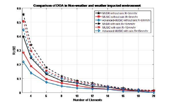
210                                                                                 Nxumalo and Walingo

signals coming from other direction than desired. Both methods involve spectrum evaluation followed
by finding the local maxima that give the estimated DOA. However, these methods are highly dependent
on physical antenna aperture array size resulting in poor resolution and accuracy [2, 4]. In addition,
they do not exploit the structure of the narrowband input data model of the measurements.
     Subspace techniques conduct characteristic decomposition of the covariance matrix for any array
output data, resulting in a signal subspace orthogonal with to noise subspace corresponding to the signal
components. Estimation of DOA is performed from one of these subspaces, assuming that noise in each
channel is highly uncorrelated. The popularity of the MUSIC algorithm [5] is due to its generality. It
is applicable to arrays of arbitrary but known configuration and response, used to estimate multiple
parameters per source. MUSIC algorithm has the ability to simultaneously measure multiple signals
with high precision and resolution among others. However, the conventional MUSIC algorithm requires
a priori knowledge of the second-order spatial statistics of the background noise and interference field.
It also involves a computationally demanding spectral search over the angle, therefore, expensive in
implementation. The ESPRIT [6] is a computationally efficient and robust subspace method of DOA
estimation. It uses two identical matched array pairs aiding it in reducing complexity. Although
ESPIRIT alleviates the computational complexity of MUSIC algorithm, it is more prone to errors [10].
Other algorithms also exist for DOA estimation. The development and performance evaluation of
these algorithms and their variants has been exhaustively done for the legacy communication network
environments [4, 7–10] and need not be reemphasised.
     The increasing demand on mobile broadband services has led to the scarcity of radio spectrum
due to spectrum exhaustion [11]. This has led to migration to higher frequency millimetre-wave
(mmW) bands, which range from 30 GHz to 300 GHz, for mmW communication with additional large
bandwidths. Apart from the merits of expanded bandwidth and high frequency reuse packing due
to shorter wavelengths, mmW communication, possess its own challenges including large path loss
suffered by mmW signals, and the effect of the weather effectors to signals in this band. Rainfall is a
common weather phenomenon that affects signal transmission at this band. In link budget planning
and design at lower frequencies, rainfall is considered as a fixed propagation attenuation [12]. The
transmitted signal suffers from absorption from the rain causing signal attenuation. In mmW systems,
the wavelengths of the signals are comparable to the raindrop size from 0.1 mm to 10 mm [13]. Hence,
apart from attenuation, the signals undergo scattering when being transmitted through rain leading to
both amplitude attenuation and phase fluctuation [14]. Rain attenuation and scattering are a function of
the rain rate, polarization, physical size of drops and operating frequency [15, 16]. Rainfall attenuation,
frequency attenuation, and phase distortion affect the received signal. For these mmW systems, DOA
algorithms that do not consider the effect of the weather are not realistic. This work is among the first
that investigates the performance of the DOA algorithms in a rainfall-impacted network and develops
a hybrid algorithm to combat the rainfall effects in DOA estimation. A realistic Markovian rainfall
channel model is used to accurately capture the rainfall variations in three cases; widespread, shower
and thunderstorm rain events.
     The rest of the paper is organized as follows. In Section 2, the system model is presented. Section 3,
represents the weather channel parameter modelling. The proposed method of efficiently estimating the
DOA and other conventional and subspace DOA estimation algorithms are presented in Section 4.
In Section 5, the performance measures and overall performance evaluation algorithm is done while
simulation results and discussion are presented in Section 6. The paper concludes in Section 7.
     Notation: The bold upper and lower-case letters represent the matrices and column vectors,
respectively. I is an identity matrix. The following superscripts (.)∗ , (.)H , (.)−1 and (.)T represent
optimality, Hermitian, inverse and transpose operators, respectively and E(.) is the mathematical
expectation, d is the spacing difference between array elements, c is the speed of light and λ is the
wavelength.

2. SYSTEM MODEL

The DOA algorithms estimate the angle of arrival of all incoming signals. In Figure 1 a uniform linear
array (ULA) of N equally spaced sensors is shown. A source transmits signals s(t) that after passing
through a weather-impacted environment arrives at the antenna at an angle θ. The signals x(t) induced
Progress In Electromagnetics Research C, Vol. 95, 2019                                                 211

Figure 1. System model.

on the antenna arrays are multiplied by adjustable complex weights w and then combined to form the
system output y(t). The processor receives array signals, system output, and direction of the desired
signal as additional information. In our model, for a wavefront narrow band signal si (t), the received
signal xi (t) at antenna element, i = 1, 2, . . . , N , is given by
                                            N

                                 xi (t) =         αi si (t)ai (θi + Δθi ) + vi (t),                    (1)
                                            i=1
where αi is the rainfall attenuation, θi the angle of arrival, Δθi the rainfall angle deviation, and vi the
measured noise at antenna i. The response function of the array element i to the signal source ai (θ̂i ) is

                                                             2πd sin θ̂i
                                   ai (θ̂i ) = exp −j(i − 1)               ,                            (2)
                                                                 λ
where λ is the wavelength, and d is the spacing difference between array elements. The total received
signal vector X(t) is expressed as:
                                        X(t) = A(θ̂)S̃(t) + V (t),                                     (3)
where
                                  X(t) = [x1 (t), x2 (t), . . . , xN (t)]T ,
                                  A(θ̂) = [a1 (θ̂1 ), a2 (θ̂2 ), . . . , aN, (θ̂I )]T ,
                                  S̃(t) = [s̃1 (t), s̃2 (t), . . . , s̃N (t)]T ,
                                  V (t) = [v1 (t), v2 (t), . . . , vN (t)]T .                          (4)
In Equation (4), s̃i (t) = αi si (t) and θ̂i = θi + Δθi . The modelling and investigation of the rainfall
attenuation αi and angle deviation Δθi due to the weather impacted rainfall channel are done in the
next section.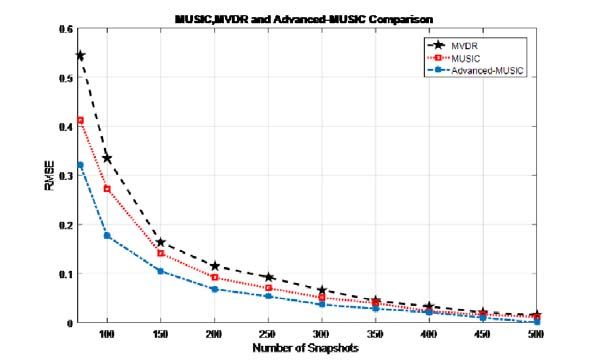
212                                                                                 Nxumalo and Walingo

3. WEATHER CHANNEL PARAMETER MODELLING

3.1. Rainfall Modeling
The magnitude of attenuation experienced by signals depends on the rain intensity. Based on its
intensity, a rain event may be classified as drizzle (D), widespread (W), shower (S), or thunderstorm
(T). The rainfall is modelled by four or fewer states of a Markov Chain, R, given by
                                               R = {D, W, S, T },                                      (5)
Table 1 presents the rain event intensities.

Table 1. Rain rates categories.

                         Description      Rain Rate (r )       Steady State (πn )
                            Drizzle             1–5                   πD
                          Widespread           5–10                   πW
                            Shower            10–40                   πS
                         Thunderstorm         > 40                    πT

    Practical rainfall, widespread, shower and thunderstorm events consist of a mix of the different rain
events [17]. This work utilizes Markov models developed from actual rain data to model practical rain
events, with the transition diagram and state transition probabilities as given bellow:
 i) Widespread rainfall: Consists of drizzle and widespread events. The transition diagram shown
                                                        W , form states i to j, with i, j ∈ R, given by
    in Figure 2, with the transitional probabilities, Pi,j
    Equation (6)
                                           W       PDD PDW
                                         Pi,j =                  ,                                   (6)
                                                  PW D PW W
      where PDW is the probability of transition from drizzle to widespread, PW D the probability of
      transition from widespread to drizzle, PDD the probability of no transition from drizzle, and PW W
      the probability of no transition from widespread.

Figure 2. Widespread rainfall.

 ii) Shower rainfall consists of drizzle, widespread and shower events. The transition diagram shown
                                                         S , form states i to j, with i, j ∈ R, given by
     in Figure 3, with the transitional probabilities, Pi,j
     Equation (7)                               ⎡                   ⎤
                                                  PDD PDW PDS
                                           S
                                         Pi,j = ⎣PW D PW W PW S ⎦ ,                                   (7)
                                                  PSD PSW PSS
      where PDS is the transition probability from drizzle to shower, PW S the transition probability from
      widespread to shower, PSD the transition probability from shower to drizzle, PSW the transition
      probability from shower to widespread, and PSS the no transition probability from shower.
Progress In Electromagnetics Research C, Vol. 95, 2019 213
Figure 3. Shower rainfall. Figure 4. Thunderstorm rainfall.
iii) Thunderstorm rainfall consists of drizzle, widespread, shower and thunderstorm events. The
T , form states i to
transition diagram shown in Figure 4, with the transitional probabilities, Pi,j
j, with i, j ∈ R, given by Equation (8)
⎡ ⎤
PDD PDW PDS PDT
⎢PW D PW W PW S PW T ⎥
T
Pi,j =⎢⎣ PSD PSW PSS PST ⎦ ,
⎥ (8)
PT D PT W PT S PT T
where PDT is the probability of transition from drizzle to thunderstorm, PW T the probability
of transition from widespread to thunderstorm, PST the probability of transition from shower
to thunderstorm, PT D the probability of transition from thunderstorm to drizzle, PT W the
probability of transition from thunderstorm to widespread, PT S the probability of transition from
thunderstorm to shower, and PT T the no transition probability from thunderstorm. The transitional
probabilities used are practically obtained from [17]. The steady state probability of an event
n, πn = {πD , πW , πS , πT }, is solved by the standard Markov chain solution methods. The expected
rate for a rainfall occurrence is derived from the probabilities as
E[r] = rn πn , (9)
n
where rn is the median rain event, and πn is the steady state probability of the nth state of the
Markov model. The actual rain rate r is computed from a lognormal distribution with the given
mean [17–19].
3.2. Attenuation Model
We consider a radio propagation environment where the signal is affected by attenuation due to the
weather-impacted factors. The total attenuation AT is given by
AT = αi + Lf s , (10)214 Nxumalo and Walingo
where αi is the rain attenuation. The ITU rainfall model [20] is used for attenuation as
αi = kr a , (11)
where r is the rain rate in mm/hr of Section 3.1. The constant parameter k and exponent a depend
on the frequency f (GHz), the polarization state, and the elevation angle of the signal path. Free space
loss attenuation, Lf s , is given by
4πd
Lf s = 20 ∗ log10 , (12)
λ
where λ is the signal wavelength in metres, and d is the distance from the transmitter.
3.3. Angle Deviation Model
The weather related factors result in the delay and scattering of the transmitted signal as well as phase
angle and angle deviation change. The angle deviation, Δθi , is modelled as a normal distributed random
variable with a mean μθ bounded as follows
Δθmin ≤ Δθi ≤ Δθmax , (13)
where Δθmin and Δθmax are the minimum and maximum angle deviations, respectively. The mean μθ
is derived from the normalised rain rate
r
μθ = , (14)
rmax
and rmax is the maximum rain rate. The assumption is reasonable as the heavier the rain, the more
the scattering. Though the weather elements affect the mean and the standard deviation, we keep the
standard deviation constant.
4. DOA ESTIMATION ALGORITHMS
4.1. MVDR Algorithm
The MVDR algorithm minimizes the output power and constrains the gain of the direction of desired
signal to unity [21] as follows,
min E{| yn (t) |2 } = min{wH σ(x, x)w}, (15)
subject to w · a(θ̂) = 1 where
yn (t) = wH σ(x, x)w, (16)
is the output of the array system, w the weight vector, H the Hermitian matrix, a(θ̂) the steering vector,
and σ(x, x) covariance matrix of the received signal x. The covariance matrix σ(x, x) is given by
N
1 H
σ(x, x) = xx , (17)
N
i=1
where N is the number of elements. From the block diagram of Figure 1, the signal vector x(t) defined
at different angles θ̂i induced on the antenna arrays is multiplied by weight vectors w and then combined
to form the system output y(t). The weighted vector w is obtained by using Lagrange multiplier in
Eq. (15) as
(σ(x, x))−1 a(θ̂)
w= . (18)
aH (θ̂)(σ(x, x))−1 a(θ̂)
Thus, MVDR computed as a Capon’s output power spectrum is given by
1
PM V DR (θ̂) = . (19)
aH (θ̂)(σ(x, x))−1 a(θ̂)
The MVDR technique is summarized in Algorithm 1.Progress In Electromagnetics Research C, Vol. 95, 2019 215
Algorithm 1 MVDR algorithm
1: Input: x = {xi (t)} = f (αi , θ̂i ), N, d, λ, K and μ ← step size
2: Compute the weight vector w, Equation (18)
3: Compute covariance matrix σ(x, x), Equation (17)
4: Compute the output array system, Equation (16)
5: Minimize the output power, Equation (15), subject to w · a(θ̂) = 1
6: Compute spectrum function, Equation (19), spanning θ
4.2. MUSIC Algorithm
MUSIC is a high-resolution subspace DOA algorithm where an estimate σ(x, x) of the covariance matrix
is obtained and its eigenvectors decomposed into orthogonal signal and noise subspace [22]. The DOA
is estimated from one of these subspaces. The noise in each channel is assumed uncorrelated. The
algorithm searches through the set off all possible steering vectors to find the ones orthogonal to the
noise subspace. The diagonal covariance matrix σ(x, x) is given by Eq. (17). The covariance matrix is
decomposed to
σ(x, x) = A(θ̂i )S̃i (t)A(θ̂i )H + σ 2 I = QΛQH , (20)
where A(θ̂i ) = [a1 (θ̂1 ), a2 (θ̂2 ), . . . , aN (θ̂I )]T is a M × D array steering matrix, σ 2 the noise variance, I
an identity matrix of size M × M , and S̃i (t) the received signal with Q unitary and a diagonal matrix
Λ = diag{λ1 , λ2 , . . . , λM }, of real eigenvalue ordered as λ1 ≥ λ2 ≥ . . . ≥ λM ≥ 0. The vector that is
orthogonal to A is the eigenvector of R having the eigenvalues of Λ. The MUSIC spatial spectrum is
defined by
1
PM U SIC (θ̂) = , (21)
aH (θ̂)Qn QH
n a(θ̂)
where a(θ̂) is the steering vector corresponding to one of the incoming signals, and Qn is the signal
substance. The MUSIC technique is summarized in Algorithm 2.
Algorithm 2 MUSIC algorithm
1: Input: x = {xi (t)} = f (αi , θ̂i ), N, d, λ, K
2: Compute covariance matrix σ(x, x), Equation (17)
3: Decomposition σ(x, x) into eigenvectors and eigenvalues in Equation (20)
4: Rearrange the eigenvectors and eigenvalues into the signal subspace and noise subspace
5: Compute the spectrum function (21) by spanning θ
6: Determine the substantial peaks of PM U SIC (θ) to acquire estimates of the angle of arrival
4.3. Proposed A-MUSIC Algorithm
In rain impacted mmW systems, the SNR is low leading to small signal intervals. The existing MVDR
and MUSIC algorithms are adversely affected and need modifications. We propose an A-MUSIC
algorithm that repeatedly reconstructs the covariance matrix to continuously obtain two noise and
signal subspaces averaged over several iterations. The reconstructed covariance matrix σ̂(x, x) is given
by
σ̂(x, x) = σ(x, x) + Jσ(x, x)∗ J, (22)
where J is MATLAB constructions given as J = f liplr(eye(N )) which returns columns flipped in
the left-right direction, and N is the number of elements. The eigen decomposition on reconstructed
covariance matrix σ̂(x, x) is
σ̂(x, x) = Q̂ΛQ̂H = QS1 ΛS1 QH H
S1 + QN 1 ΛN 1 QN 1 , (23)216 Nxumalo and Walingo
where σ̂(x, x) is divided into signal subspace QS and noise subspace QN . Using low rank of matrix
instead of full rank matrix σ̂(x, x) can be reconstructed into ωx as
ωx = QS2 ΛS2 QH H
S2 + QN 2 ΛN 2 QN 2 . (24)
The average signal subspace (QS ), signal eigenvalue (ΛS ), noise subspace (QN ), and the noise eigenvalue
(ΛN ) are given by
QS1 + QS2
QS = ,
2
QN 1 + QN 2
QN = ,
2
ΛS1 + ΛS2
ΛS = ,
2
ΛN 1 + ΛN 2
ΛN = . (25)
2
The A-MUSIC spectrum is then defined by
(σ(s,s))(σ(s,s))H
aH (θ̂) N a(θ̂)
P(A-M U SIC)(θ̂) = , (26)
aH (θ̂)σ(n, n)a(θ̂)
where σ(s, s) = QS Λ−1 H −1 H
S QS , and σ(n, n) = QN ΛN QN are signal and noise subspace covariance matrix.
The A-MUSIC technique is summarized in Algorithm 3.
Algorithm 3 Proposed A-MUSIC Algorithm
1: Input: x = {xi (t)} = f (αi , θ̂i ), N, d, λ, K
2: Compute the covariance matrix, Equation (20)
3: Compute reconstructed covariance matrix σ̂(x, x), Equation (22)
4: Compute the Eigen decomposition on reconstructed covariance matrix σ̂(x, x)
5: Compute reconstructed covariance matrix ωx , for Equation (24)
6: Compute the average signal subspace, noise subspace, signal eigenvalues, and the noise eigenvalue,
QS , QN , ΛS , ΛN Equation (25)
7: Determine signal and noise subspace averaged covariance matrix σ(s, s) and σ(n, n)
8: Compute the spectrum function, Equation (26), spanning θ
5. PERFORMANCE MEASURES
The performance of the DOA estimation algorithms is evaluated in terms of spectrum functions,
Equations (19), (21), and (26), Root Mean Square Error (RMSE), and signal to noise ratios. The
RMSE is given by
K N
1
RM SE = (θ̃i j − θi )2 , (27)
K ∗N
j=1 i=1
where K is the number of simulation trials; N is the number of elements; and the estimate of the ith
angle of arrival in the jth trial is θ̃ij . The signal to noise ratio (SNR) is given by
x
SN R = 20 log 10 , (28)
v
where x is the received signal strength in dB, and v is the noise strength in dB. The overall performance
evaluation is done as in algorithm 4.
The complexity of MVDR and MUSIC algorithm has been derived as shown in Table 2 [23, 24].
For A-MUSIC, there are three major computational steps needed to estimate the DOA. The complexityProgress In Electromagnetics Research C, Vol. 95, 2019 217
Algorithm 4 System Algorithm
1: Input: Required rainfall
2: Compute expected rain rate, equation
3: Compute the actual rain rate r from lognormal distribution with given mean
4: for i number of antennas < Nmax
5: Compute the rain attenuation αr , total attenuation given
6: AT and the angle θ̂i . find the angle deviation Δθi as shown
7: in (13) and the mean μθ .
8: Determine the received signal xi (t).
9: end for
10: Determine DOA, Algorithm 1, 2 and 3.
of the first step is the covariance function and reconstruction of the covariance matrix, O(N 2 K). The
second step is the eigen-value decomposition operation, which has a complexity of O(N 3 ). The third
step is obtaining the spatial pseudo spectrum, which has a complexity of O(Jθ · JΔθ (N + 1)(N − K)/2),
with J being the number of spectral points of the total angular field of view. Therefore, the total
complexity of A-MUSIC is given by O(N 2 K + N 3 ) + O(Jθ · JΔθ (N + 1)(N − K)/2).
Table 2. Computational complexity of DOA estimation algorithms.
DOA Algorithm Computational Complexity
MVDR O(N 2 K + N 3 + (2N 2 + 3N ))
MUSIC O(N 2 K + N 3 + JN )
A-MUSIC O(N 2 K + N 3 ) + O(Jθ · JΔθ (N + 1)(N − K)/2)
6. RESULTS AND DISCUSSION
The performances of the general MVDR, MUSIC, and the proposed algorithm A-MUSIC are investigated
and discussed in this section. The performance of the algorithms for different numbers of array elements,
rain rates, and SNR is investigated. Unless otherwise specified for a particular result, the simulation
parameters are as given in Table 3. The developed results are for a case where four signals impinge
on the ULA sensors from the same signal source. The signal consists of the first direct path signal
and the scaled and delayed replicas of the first signal representing multipath signals known priori. The
background noise is modelled as a stationary Gaussian white random process.
The results of Figures 5(a)–(d) show the spatial output spectrum in dB’s of the MVDR, MUSIC
and the proposed A-MUSIC for different rain rates from zero to 20 mm/hr representing the following
cases; no rain, widespread, shower and thunderstorm rain conditions with the number of elements N = 5
for 100 snapshots. Note that without rain the spectrum results for MVDR and MUSIC are similar to
the ones in [25], respectively. From the results, the following can be observed; the accuracy of DOA
estimation decreases with increasing rain rate, and the performance of the A-MUSIC is better than
MUSIC followed by MVDR. This is because of the multiple averaging nature of A-MUSIC algorithm.
It can also be observed that at a higher rain rate of 20 mm/hr MVDR and MUSIC fail to estimate the
direction of arrival.
To analyse the performance of the DOA algorithms and the proposed method, a simulation was
done for four neighbouring signals, and the results are tabulated in Table 4. The results depict the
accuracy of the three DOA algorithms. There is a degradation in accuracy for the developed algorithm
as the rain rate increases. From zero to 20 mm/hr the degradation of MVDR is 47%, for MUSIC is
33%, and for A-MUSIC is 3.3% at reference point −20 dB.218 Nxumalo and Walingo
Table 3. Simulation parameters for MVDR, MUSIC and A-MUSIC algorithm.
Simulation Parameters Values
Input θ [00 , 100 , 350 , 600 ]
Number of elements N = 5, N = 15
Spacing difference d = 0.5λ
Signal-to-noise ratio SN R = 20 dB
Snapshots K = 100
Rain rate in (mm/h) [0, 2.5, 6, 12, 20]
a at f (GHz) 0.7103
k at f (GHz) 1.16995
Δθmin , Δθmax [00 − 650 ]
Table 4. Spectrum performance for actual DOA = [00 , 100 , 350 , 600 ].
Figure 5(a) Estimated DOA Error %
MVDR 0.02010 , 9.90 , 35.010 , 59.80 3.372
MUSIC 0.020 , 10.0010 , 35.020 , 600 2.067
A-MUSIC 00 , 100 , 350 , 600 0
Figure 5(b) Estimated DOA Error %
MVDR −0.0320 , 9.80 , 34.00 ,58.80 10.057
MUSIC 1.20 , 10.50 , 34.780 , 60.10 17.796
A-MUSIC 0.0010 , 100 , 350 , 600 0.1
Figure 5(c) Estimated DOA Error %
MVDR 0.220 , 9.50 , 34.760 , 620 31.018
MUSIC 0.10 , 10.30 , 34.80 , 61.10 15.404
A-MUSIC 0.0010 , 10.0020 , 35.030 , 60.010 0.2217
Figure 5(d) Estimated DOA Error %
MVDR −0.320 , 11.10 , 35.70 , 63.20 50.33
MUSIC 0.20 , 10.20 , 36.00 , 63.00 29.86
A-MUSIC 0.010 , 10.20 , 35.10 , 60.010 3.303Progress In Electromagnetics Research C, Vol. 95, 2019 219
(a) (b)
(c) (d)
Figure 5. DOA estimation attenuation for N = 5 with various rainfall rates. (a) DOA estimation
attenuation with rain rate r = 0 mm/hr for N = 5. (b) DOA estimation attenuation at drizzle rain
rate r = 2 mm/hr for N = 5. (c) DOA estimation attenuation at widespread rain rate r = 8 mm/hr for
N = 5. (d) DOA estimation attenuation at shower rain rate r = 20 mm/hr for N = 5.
Similarly, the results of Figures 6(a)–(d) show the spatial output power spectrum in dB’s of the three
algorithms discussed in Section 4 for different rain rates representing no rain, widespread, shower and
thunderstorm rain conditions. However, the number of elements N = 15 for 100 snapshots. Note that
without rain the spectrum results for MVDR and MUSIC are similar to the ones in [26, 27], respectively.
The results reinforce the notion that the accuracy of DOA estimation decreases with increasing rain
rate, and the performance of the A-MUSIC is better than MUSIC followed by MVDR.
The results of estimated DOAs are tabulated in Table 5. Similarly, the results depict the accuracy
of the three DOA algorithms. There is a degradation in accuracy for the developed algorithm as the
rain rate increases. From zero to 20 mm/hr, the degradation of MVDR is 38%, for MUSIC is 23%, and
for A-MUSIC is 1.23% at reference point −20 dB.
For different numbers of antennas, comparison of the results in Figures 5(a)–(d) for N = 5 and
Figures 6(a)–(d) for N = 15 is done. We observe that DOA estimation improves with increasing the
number of antenna elements. At the −40 dB reference point, we observe that the width of the spectrum
function is wide, leading to high error estimation of the angle of arrival.
The results of Figure 7 represent the RMSE value vs rain rate at a different angle of arrival
[200 , 400 , 500 ] for two different reference spectrum function levels −20 dB and −40 dB with N = 10.
As expected, the RMSE increases with an increase in rain rate. It is also higher at −40 dB than
−20 dB. The performance order of the algorithms is MVDR, MUSIC, and A-MUSIC. Similarly, the
results of Figures 8(a)–(c) represent the RMSE error comparison for different rain conditions albeit at220 Nxumalo and Walingo
(a) (b)
(c) (d)
Figure 6. DOA estimation attenuation for N = 15 with various rainfall rates. (a) DOA attenuation
with rain rate r = 0 mm/hr for N = 15. (b) DOA attenuation in light rain rate of r = 2 mm/hr for
N = 15. (c) DOA attenuation in moderate rain rate of r = 8 mm/hr for N = 15. (d) DOA attenuation
in heavy rain rate of r = 20 mm/hr for N = 15.
Figure 7. MUSIC, MVDR and A-MUSIC accuracy comparison at −20 dB and −40 dB with DOA =
[200 , 400 , 500 ].Progress In Electromagnetics Research C, Vol. 95, 2019 221
Table 5. Spectrum performance for actual DOA = [00 , 100 , 350 , 600 ].
Figure 6(a) Estimated DOA Error %
MVDR 00 , 10.0010 , 35.020 , 60.010 0.5977
MUSIC 0.0020 , 10.010 , 35.010 , 60.020 0.3623
A-MUSIC 00 , 100 , 350 , 600 0
Figure 6(b) Estimated DOA Error %
MVDR 0.20 , 10.10 , 33.70 , 59.60 25.381
MUSIC 0.010 , 10.20 , 34.70 , 60.10 4.024
A-MUSIC 0.0010 , 10.010 , 35.010 , 600 0.2286
Figure 6(c) Estimated DOA Error %
MVDR 0.230 , 9.60 , 35.30 , 57.50 32.024
MUSIC 0.10 , 10.20 , 35.010 , 60.010 12.0453
A-MUSIC 0.010 , 100 , 350 , 600 1.0
Figure 6(d) Estimated DOA Error %
MVDR −30 , 9.50 , 34.50 , 58.50 38.929
MUSIC −20 , 10.20 , 35.10 , 59.50 23.00
A-MUSIC 0.0020 , 9.90 , 35.010 , 600 1.2286
variable antenna elements N = 5, N = 10, and N = 20 for SN R = 20 dB. The RMSE increases with
increase in rainfall, and the proposed A-MUSIC performs better than the other models due to repeatedly
reconstruction of the covariance matrix to obtain two noise and signal subspaces continuously that are
averaged for several iterations. An additional deduction from the result is that the RMSE errors decrease
with the increase in antenna elements.
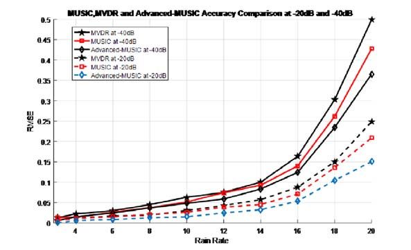
To reiterate the deduction from Figures 8(a)–(c), Figure 9 presents the results of the RMSE error vs
(a) (b)222 Nxumalo and Walingo
(c)
Figure 8. DOA estimation attenuation error comparison. (a) DOA estimation attenuation error
comparison for N = 5. (b) DOA estimation attenuation error comparison for N = 10. (c) DOA
estimation attenuation error comparison for N = 20.
Figure 9. Comparison of DOA estimation algorithms in non-weather and weather impacted
environment.
Figure 10. Error comparison in various rain rates vs SNR.Progress In Electromagnetics Research C, Vol. 95, 2019 223
the number of elements for no rain and the rate of 15 mm/hr. It can be observed that as the number of
elements increases the RMSE decreases. Still the proposed A-MUSIC outperforms MVDR and MUSIC
algorithms in terms of error comparison. We conclude that the statistical channel model proposed in this
paper is highly recommended in both rainfall and non-rainfall regions due to its excellent performance.
To further investigate the performance of the system, the DOA estimation algorithms are tested at
different rain rates leading to different SNR conditions and results presented in Figure 10 for N = 10.
As expected, the RMSE decreases with an increase in the values SNR, and A-MUSIC outperforms
MVDR and MUSIC making it highly recommended in estimation of DOA in both normal and rainfall
environments.
Figure 11 shows the performance comparison in rainfall for various numbers of snapshots at
SN R = 20 dB, r = 20 mm/hr, and N = 5. As expected, the RMSE decreases as we increase the
number of trials from 100 to 500. Therefore, increasing number of simulation trials can improve the
performance of the algorithms. It can be intuitively observed that the proposed A-MUSIC surpasses the
MVDR and classical MUSIC estimator over the range of the number of snapshots that we simulated.
Figure 11. Error comparison in RMSE vs number of snapshots.
7. CONCLUSION
This work has investigated the performance of the existing DOA algorithms, MVDR, and MUSIC
compared with our proposed A-MUSIC on a weather-impacted network. The investigation is conducted
for conditions of no rain, widespread, shower and thunderstorm rainfall. The deduction from the
investigation indicates that the algorithms performance accuracy degrades by up to 43% and 28%
for MVDR and MUSIC, respectively, from no rain condition to thunderstorm rainfall condition with
MUSIC performing better than MVDR. The RMSE performance of the algorithms is shown to decrease
by increasing the values of SNR and number of antenna elements. The work develops an A-MUSIC
algorithm for the weather impacted conditions. The performance of the developed A-MUSIC is
superior to the existing algorithm in terms of accuracy and RMSE parameters. The performance
accuracy degrades by up to 2.3% from no rain condition to thunderstorm rainfall condition. However,
its complexity is higher than the other algorithms. This work opens further investigation into the
performance of DOA algorithms in weather impacted environment and the need for redesign of the
existing algorithms. The accuracy of the investigation could be validated further by the derivation of
the Cramer-Rao lower bounds and other statistical measures.
REFERENCES
1. Tsoulos, G. V., “Smart antennas for mobile communication systems: Benefits and challenges,” IEE
Electron. Commun Eng. Journal, Vol. 11, No. 2, 84–94, April 1999.224 Nxumalo and Walingo
2. Lavate, T. V., V. K. Kokate, and A. M. Sakpal, “Performance analysis of MUSIC and ESPRIT
DOA estimation algorithms for adaptive array smart antenna in mobile communication,” Proc. of
IEEE, Second Int. Conf. Computer and Network Technology, 308–311, 2010.
3. Shaukat, S. F., H. Mukhtar, R. Farooq, H. U. Saeed, and Z. Saleem, “Sequential studies of
beamforming algorithms for smart antenna systems,” World Applied Sciences Journal, Vol. 6,
No. 6, 754–758, 2009.
4. Balanis, C., Antenna Theory: Analysis and Design, 3rd Edition, John Wiley and Sons, Hoboken,
New Jersey, 2005.
5. Leon De, F. A. and S. J. J Marciano, “Application of MUSIC, ESPRIT and SAGE algorithms for
narrowband signal detection and localization,” TENCON, IEEE Reg. 10 Conf., 1–4, 2006.
6. Qian, C., H. Lei, and H. C. So, “Computationally efficient ESPRIT algorithm for direction-of-arrival
estimation based on Nyström method,” Signal Processing, Vol. 94, 74–80, 2014.
7. Xu, C. and J. Krolik, “Space-delay adaptive processing for MIMO RF indoor motion mapping,”
IEEE. Int. Conf. on Acoustics, Speech and Signal Processing (ICASSP), 2349–2353, Brisbane,
QLD, April 2015.
8. Dhope, T., D. Simunic, and M. Djurek, “Application of DOA estimation algorithms in smart
antenna systems,” Studies in Informatics and Control, Vol. 19, No. 4, 445–452, December 2010.
9. Schmidt, R., “Multiple emitter location and signal parameter estimation,” IEEE Transactions on
Antennas and Propagation, Vol. 34, No. 3, 276–280, 1986.
10. Roy, R. and T. Kailath, “ESPRIT-a subspace rotational approach to estimation of parameters of
cissoids in noise,” IEEE Transactions on Acoustics, Speech, and Signal Processing, Vol. 34, No. 10,
1340–1342, 1986.
11. Zhang, Y., P. Wang, and Goldsmith, “Rainfall effect on the performance of millimeter-wave MIMO
systems,” IEEE Transactions on Wireless Communications, Vol. 14, No. 9, 4857–4866, September
2015.
12. Pi, Z. and F. Khan, “An Introduction to millimeter-wave mobile broadband systems,” IEEE
Commun. Mag., Vol. 49, No. 6, 101–107, June 2011.
13. Ishimaru, A., Wave Propagation and Scattering in Random Media, IEEE Press, Piscataway, NJ,
USA, 1978.
14. Ishimaru, A., S. Jaruwatanadilok, and Y. Kuga, “Multiple scattering effects on the radar cross
section (RCS) of objects in a random medium including backscattering enhancement and shower
curtain effects,” Waves Random Media, Vol. 14, 499–511, 2004.
15. Agber, J. U. and J. M. Akura, “A high-performance model for rainfall effect on radio signals,”
Journal of Information Engineering and Applications, Vol. 3, No. 7, 1–12, 2013.
16. Calla, O. and J. Purohit, “Study of effect of rain and dust on propagation of radio waves at
millimeter wavelength,” International Centre for Radio Science, 1–4, ‘OM NIWAS’A-23 Shastri
Nagar Jodhpur, January 1990.
17. Alonge, A. A. and T. J. Afullo, “Fractal analysis of rainfall event duration for microwave
and millimetre networks: Rain queueing theory approach,” IET Microwaves, Antennas and
Propagation, Vol. 9, No. 4, 291–300, 2015.
18. Kedem, B. and L. S. Chiu, “On the lognormality of rain rate,” Proceedings of the National Academy
of Sciences, Vol. 84, No. 4, 901–905, 1987.
19. Cho, H. K., K. P. Bowman, and G. R. North, “A comparison of gamma and lognormal distributions
for characterizing satellite rain rates from the tropical rainfall measuring mission,” Journal of
Applied Meteorology, Vol. 43, No. 11, 1586–1597, 2004.
20. I.T.U. Radiowave Propagation Series, “Specific attenuation model for rain for use in prediction
methods,” Rec. P.838-3, ITU-R, Geneva, Switzerland, 2005.
21. Oh, D., Y. Ju, and J. Lee, “An improved MVDR-like TOA estimation without EVD for high-
resolution ranging system,” IEEE Communications Letters, Vol. 18, No. 5, 753–756, May 2014.
22. El Gonnouni, A., M. Martinez-Ramon, J. L. Rojo-Alvarez, G. Camps-Valls, A. R. Figueiras-Vidal,
and C. G. Christodoulou, “A support vector machine MUSIC algorithm,” IEEE Transactions onProgress In Electromagnetics Research C, Vol. 95, 2019 225
Antennas and Propagation, Vol. 60, No. 10, 4901–4910, October 2012.
23. Balakrishnan, S. and L. T. Ong, “GNU radio based digital beamforming system: BER
and computational performance analysis,” Proc. of the 2015 23rd European Signal Processing
Conference (EUSIPCO), 1596–1600, Nice, France, August 31–September 4, 2015.
24. Stoeckle, C., J. Munir, A. Mezghani, and J. A. Nossek, “DOA estimation performance and
computational complexity of subspace- and compressed sensing-based methods,” Proc. in WSA
2015 19th International ITG Workshop on Smart Antennas, 1–6, March 2015.
25. Bhaumik, B., “Performance analysis of MUSIC algorithm for DOA estimation,” International
Research Journal of Engineering and Technology (IRJET), Vol. 4, 1667–1670, February 2017.
26. Aboul-Seoud, A. K., A. K. Mahmoud, A. Hafez, and A. Gaballa, “Minimum variance variable
constrain DOA algorithm,” PIERS Proceedings, 798–803, Guangzhou, China, August 25–28, 2014.
27. Kokare, R. G. and V. S. Hendre, “Estimation of direction of arrival using music and esprit algorithm
for smart antenna,” International Journal of Control Theory and Applications, Vol. 10, No. 38,
2017.You can also read