CAUSAL-EFFECT ANALYSIS USING BAYESIAN LINGAM COMPARING WITH CORRELATION ANALYSIS IN FUNCTION POINT METRICS AND EFFORT - IJMEMS
←
→
Page content transcription
If your browser does not render page correctly, please read the page content below
International Journal of Mathematical, Engineering and Management Sciences
Vol. 3, No. 2, 90–112, 2018
ISSN: 2455-7749

       Causal-Effect Analysis using Bayesian LiNGAM Comparing with
          Correlation Analysis in Function Point Metrics and Effort
                                   Masanari Kondo*, Osamu Mizuno†
                                        Kyoto Institute of Technology
                                                Kyoto, Japan
                            E-mails: *m-kondo@se.is.kit.ac.jp, †o-mizuno@kit.ac.jp
                                           †
                                             Corresponding author

                                                 Eun-Hye Choi†
                  National Institute of Advanced Industrial Science and Technology (AIST)
                                             Ikeda, Osaka, Japan
                                          E-mail: e.choi@aist.go.jp

                              (Received March 31, 2017; Accepted September 27, 2017)

Abstract
Software effort estimation is a critical task for successful software development, which is necessary for appropriately
managing software task assignment and schedule and consequently producing high quality software. Function Point
(FP) metrics are commonly used for software effort estimation. To build a good effort estimation model, independent
explanatory variables corresponding to FP metrics are required to avoid a multicollinearity problem. For this reason,
previous studies have tackled analyzing correlation relationships between FP metrics. However, previous results on the
relationships have some inconsistencies. To obtain evidences for such inconsistent results and achieve more effective
effort estimation, we propose a novel analysis, which investigates causal-effect relationships between FP metrics and
effort. We use an advanced linear non-Gaussian acyclic model called BayesLiNGAM for our causal-effect analysis, and
compare the correlation relationships with the causal-effect relationships between FP metrics. In this paper, we report
several new findings including the most effective FP metric for effort estimation investigated by our analysis using two
datasets.

Keywords- Software effort estimation, Function point (FP) metrics, Causal-effect analysis, Correlation analysis, Linear
non-Gaussian acyclic model (LiNGAM), BayesLiNGAM.

1. Introduction
Software effort estimation is an important task in software development, which predicts a
necessary development cost to meet a scheduled deadline of software release. In real industrial
situations, however, many software projects fail on accurate effort estimation, and thus exceed
cost and the scheduled deadline. For instance, the chaos report (The Standish Group, 1994) points
out that on average 89% of companies are exceeding the estimated costs. In addition, Molokken
and Jorgensen (2003) report that the development time delay reaches approx. 30% and up to 40%
of the scheduled time.

To address such problems and achieve more accurate effort estimation, many effort estimation
models have been studied so far (Wen et al., 2012). Effort estimation models are often regression
models (e.g. linear regression models), and use metrics to estimate efforts. Among such metrics,
the most widely-used ones are FP (Function Point) metrics.

On the other hand, Kitchenham et al. (2007) indicate that some studies show inconsistent results
in effort estimation. For instance, Jeffery et al. (2000) report that using Cross-Company Datasets

                                                           90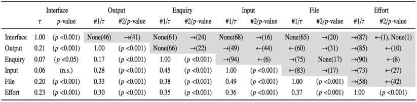
International Journal of Mathematical, Engineering and Management Sciences
Vol. 3, No. 2, 90–112, 2018
ISSN: 2455-7749

(CC) are worse than using Within-Company Datasets (WC) in effort estimation. Differently from
(Jeffery et al., 2000), Briand et al. (1999) and Mendes et al. (2005) report that CC is as good as
WC. Kitchenham et al. (2007) present a systematic review to summarize such reports. However,
it cannot determine which of WC or CC is better.

To remedy the inconsistencies among the results of different researchers, it is important to analyze
the relationships among metrics for effort estimation. The reason is that in an effort estimation
model (e.g. a linear regression model) using metrics, we get a misleading result due to the
multicollinearity problem (Farrar and Glauber, 1967) if explanation variables corresponding to the
metrics (e.g. FP metrics) are not independent. So far, a lot of studies (Kitchenham and Känsälä,
1993; Jeffery and Stathis, 1996; Lokan, 1999; Uzzafer, 2016) have investigated the relationships
between FP metrics using correlation analysis. However, they have also reported inconsistent
results that the explanation variables can be either dependent or independent (Jeffery and Stathis,
1996; Kitchenham and Känsälä, 1993).

In this paper, we propose a novel analysis that investigates causal-effect relationships between FP
metrics and effort in addition to correlations between FP metrics. Causal-effect relationships could
provide us additional information on relationships among metrics such that a certain correlation is
a spurious correlation, and some metrics do not have a correlation, however, have causal-effect
relationships with other metrics. In our study, we assume that FP metrics and effort are modeled
using a Linear Non-Gaussian Acyclic Model (LiNGAM) (Shimizu et al., 2006). In particular, we
adopt an advanced LiNGAM called BayesLiNGAM (Hoyer and Hyttinen, 2009) to identify the
causal-effect relationships between FP metrics and effort.

We address the following three research questions and obtain findings for each of them:

RQ1. Are correlation coefficients between FP metrics in our dataset similar to those in
previous research?
   The correlation coefficients in our dataset are similar to the majority results in previous
   research. Previous researches (Kitchenham and Känsälä, 1993; Jeffery and Stathis, 1996;
   Lokan, 1999; Uzzafer, 2016) investigate relationships between FP metrics, however, they have
   reported inconsistent results. Thus, we investigate the correlation in our datasets.

RQ2. How many bootstrap samples should we use?
  A sufficient sample size is 100. BayesLiNGAM occasionally extracts wrong causal-effect
  relationships. To overcome this deficiency, we adopt a general random resampling approach,
  called bootstrap sampling (Efron, 1992). Thus, we investigate this RQ to select the sufficient
  number of samples for bootstrap sampling.

RQ3. What are causal-effect relationships between FP metrics and Effort?
  The strengths of the causal-effect relationships are similar to those of the correlation
  relationships, however, the directions of the causal-effect relationships depend on datasets.

                                                 91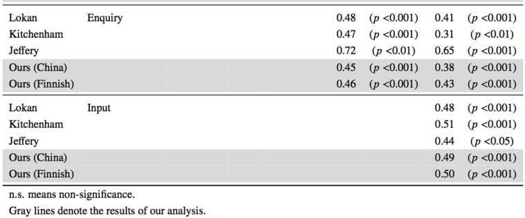
International Journal of Mathematical, Engineering and Management Sciences
Vol. 3, No. 2, 90–112, 2018
ISSN: 2455-7749
The main contributions of our paper are as follows:
We present the first investigation of the causal-effect relationships between FP metrics and
effort using two datasets.
We show that the causal-effect relationships can provide additional relationships between FP
metrics and effort.
From our results, the correlation coefficients in our dataset are similar to the majority results in
previous research. In addition, the existence of the causal-effect relationships is similar to that of
the correlation relationships, however, the directions of the causal-effect relationships depend on
datasets. Interface, one of the FP metrics, often does not have strong correlation coefficients and
causal-effect relationships with other FP metrics. However, interestingly, Interface has the causal-
effect relationships to effort. This means Interface is an independent metric. Therefore, if we use
Interface as an explained variable for an effort estimation model, Interface does not cause a
multicollinearity problem. In addition, other FP metrics except Interface have both the causal-
effect relationships and the correlation relationships with each other. Those metrics may lead a
multicollinearity problem.
The organization of this paper is as follows: Section 2 introduces related work and
BayesLiNGAM. Section 3 explains the experimental setup and used datasets. Section 4 presents
research questions and answers. Section 5 gives discussions on questions arise from the
experiment results. Section 6 describes threats to validity. Section 7 presents a conclusion and
future work.
2. Background
2.1 Motivating Example
To analyze a relationship between factor (e.g. FP metrics) using only a correlation coefficient
involves a risk. We describe a risk using the following example: In the software development, a
project sometimes falls into a runaway status (Takagi et al., 2005). An expert developer who has
a long experience is often employed to extinguish a runaway project. Then, the high effort projects
that fall into a runaway status and the projects that the expert developer belongs to are strongly
correlated, when we analyze if an effort of a project that the expert developer belongs to is either
high or low. Such a correlation can lead a misunderstanding such that the project requires a high
effort due to the expert developer, and thus we may take a wrong solution (e.g. removing the expert
developer from the project).
Therefore, it is risky to determine the reason of a high effort project using a correlation analysis
only. If we investigate a causal-effect relationship between the expert developer and the high effort
projects, we may not conclude the wrong solution. This is a motivation to use not only a correlation
analysis but also a causal-effect analysis in our approach.
2.2 Related Work
2.2.1 Effort Estimation
Software effort (shortly, effort) is a measure to indicate whole working time for the software
development. So far, various studies (Molokken and Jorgensen, 2003; Wen et al., 2012; Jorgensen
and Shepperd, 2007) have proposed effort estimation approaches. FP metrics (Albrecht and
Gaffney, 1983) are common metrics to build an effort estimation model, which are provided by
the International Function Point Users Group (IFPUG) to measure the size of software. For
92International Journal of Mathematical, Engineering and Management Sciences
Vol. 3, No. 2, 90–112, 2018
ISSN: 2455-7749
instance, Albrecht is the first person who developed a methodology of FP metrics in IBM and
(Albrecht and Gaffney, 1983) originally propose adopting FP metrics for effort estimation. Ahn et
al. (2003) present adopting FP metrics for effort estimation of software maintenance.
FP metrics measure five elementary function types to estimate a size of software; two data
functions types — internal logical files (File) and external interface files (Interface) — and three
transactional function types — external inputs (Input), external outputs (Output), and external
inquiries (Enquiry). These function types are used as explanatory variables for an effort estimation
model in a hypothesis that large-sized software requires large effort (Abran et al., 2002).
In general, the estimation model (e.g. a regression model) needs an assumption that explanatory
variables are independent (Farrar and Glauber, 1967). To confirm the assumption, many studies
(Lokan, 1999; Jeffery and Stathis, 1996; Kitchenham and Känsälä, 1993; Uzzafer, 2016) have
reported correlations between FP metrics. For instance, Kitchenham and Känsälä (1993) report FP
metrics have correlations with each other, and are not well-formed. In addition, Lokan (Lokan,
1999) indicates that results of existing research have an inconsistency.
In this paper, we first perform a correlation analysis that means, we calculate correlation
coefficients between FP metrics in our datasets, to compare with previous research. We next
calculate causal-effect relationships between FP metrics and effort for a more detailed analysis.
Finally, Kitchenham and Känsälä (1993) and Jeffery and Stathis (1996) report Pearson correlation
coefficients between FP metrics and Effort. For instance, Kitchenham and Känsälä analyze the
coefficients and use stepwise multivariate regression to build the effort estimation model. Jeffery
and Stathis report the coefficients between FP metrics and Effort, and those between Unadjusted
Function Points (UFP) and Effort. There are some inconsistent results between Kitchenham et al.
and Jeffery and Stathis differently from their work, in this paper, we use Kendall’s t B (Sprent and
Smeeton, 2016) to analyze correlation coefficients between FP metrics, and focus on causal-effect
relationships between FP metrics and Effort.
2.2.2 Causal Discovery
A causal-effect relationship is an important relationship in an engineering to estimate and solve an
industrial problem. To solve the industrial problem needs to decide if each metric is either an
explanatory variable or an objective variable to build an estimation model. The causal-effect
relationship can support the decision.
In addition, if we find out causal-effect relationships correctly, we can control values of arbitrary
metrics using an interpretation (Pearl, 2002). The interpretation is that when a variable in a certain
probability model is changed by a disturbance effect, we can observe an effect for the whole
probability model by considering a direct effect by the variable (Pearl, 2002). Consequently, in the
interpretation, we can consider the probability model whose variable can be intentionally changed
by a disturbance effect, although a correlation is a result of analyzing data, and cannot consider a
change by a disturbance effect.
To identify causal-effect relationships, we typically use a counterfactual thinking or structural
causal models (Holland et al., 1985; Robins, 1986; Hernán, 2004; Heinze-Deml et al., 2017; Pfister
et al., 2017; Shimizu et al., 2006; Hoyer and Hyttinen, 2009). Counterfactual thinking uses a
contrary fact. For instance, in counterfactual thinking, we consider two facts to identify causal-
93International Journal of Mathematical, Engineering and Management Sciences
Vol. 3, No. 2, 90–112, 2018
ISSN: 2455-7749
effect relationships: she did well on exam because she was coached by her teacher, and she did
not well on exam because was not coached by her teacher. Then, we compare these two facts to
identify that the study is causal to the result of the exam or not for her. However, it is difficult to
compare the two facts (Holland et al., 1985). Structural causal models are defined on numerical
models. For instance, Shimizu et al. (2006) use Linear, Non-Gaussian, Acyclic Model to solve
causal discovery.
In this paper, we use a type of structural causal models. The proposed approach uses a Directed
Acyclic Graph (DAG) (Pearl, 2002) to describe causal-effect relationships between factors
(metrics). To identify DAG is difficult, however, Shimizu et al. (2006) report that DAG is
identifiable when we assume a non-Gaussian disturbance density instead of Gaussian for DAG.
Fig. 1. Example causal-effect relationships among chocolate consumption, Nobel laureates and GDP
Finally, we illustrate two more motivating examples in the causal discovery. Messerli (Messerli,
2012) studies correlation relationships between chocolate consumption and Nobel laureates; there
is a strong linear correlation (r=0.791, p-valueInternational Journal of Mathematical, Engineering and Management Sciences
Vol. 3, No. 2, 90–112, 2018
ISSN: 2455-7749
that causal-effect relationships can be extracted from only observed data under certain
assumptions. One of such assumptions is the use of a Linear Non-Gaussian Acyclic Model
(LiNGAM). LiNGAM is a data-generating model satisfying the following three properties:
1. A Directed Acyclic Graph (DAG) represents a one-to-one mapping between observed
variables .
2. The value assigned to each variable xi is a linear function of the values already assigned to
the variables, plus a disturbance (noise) term ei , and plus a constant term ci , that is
xi b x ij
k ( j )k (i )
j ei ci , (1)
where k(i) is a causal order. LiNGAM calculates all possible causal orders. Thus, if we consider
many variables, the number of causal orders is explosively increased. We’ll discuss more details
of this problem in discussion section 5.6.
3. The disturbances ei are all continuous random variables. The ei are generated by non-
Gaussian distribuions of non-zero variances. The ei are independent of each other, i.e.
p(ei , , en ) i pi (ei ) .
2.4 Bayesian Discovery of Linear Acyclic Causal Models
In our approach, we extract causal-effect relationships by using the simple Bayesian inference on
LiNGAM (BayesLiNGAM) (Hoyer and Hyttinen, 2009). BayesLiNGAM calculates posterior
probabilities of possible DAGs from only given data. Posterior probabilities are calculated as
follows:
p(D | Gm )P(Gm )
P(Gm | D) , (2)
p(D)
where is the different possible DAGs, and N is the number of data samples.
D= is the observed dataset. Here P(D) is a constant that simply normalizes the
distribution. P(Gm ) is the prior probability distribution over DAGs and incorporates any domain
knowledge that we have. When we do not have any knowledge, we assume a uniform prior
probability distribution over all DAGs. The marginal likelihoods are calculated as follows:
p(D | Gm ) p(D | q , Gm ) p(q | Gm )dq , (3)
where q consists of all the parameters (i.e. the coefficients bij , the constants ci , and the
disturbance densities pi (ei ) ). p(q | Gm ) is calculated when we assume three assumptions that bij
is a standard Gaussian distribution with zero-mean and unit variance, ci is zero, and pi (ei ) models
95International Journal of Mathematical, Engineering and Management Sciences
Vol. 3, No. 2, 90–112, 2018
ISSN: 2455-7749
a parameterization of the densities. pi (ei ) implements the two quite basic parameterizations: a
simple two-parameter exponential family distribution combining the Gaussian and Laplace
distributions, and a finite mixture of Gaussian density family. The integral is calculated by the
Laplace approximation. We use this approach (Hoyer and Hyttinen, 2009) for our experiment.
Here we need to compute an approximation to (3). By the definition of LiNGAM (Hoyer and
Hyttinen, 2009), p(D | q , Gm ) is transformed to
p(D | q , Gm ) pi (xi
i
b x ij j
k ( j )k (i )
ci ). (4)
Fig. 2. Example extraction of a causal-effect relationship by BayesLiNGAM
2.5 Outputs of BayesLiNGAM
We describe outputs of BayesLiNGAM to understand analyzed data. Fig. 2 shows an example of
an output of BayesLiNGAM. First, we input two observed variables, Metric A and Metric B, to
BayesLiNGAM. Each variable has N samples data. Then, BayesLiNGAM calculates posterior
probabilities of causal-effect relationships to the all possible combinations of metrics. Posterior
probabilities provide us which causal-effect relationship has the strongest possibility. In this
example, two metrics have three possible combinations of metrics; Metric A is a cause of Metric
B, Metric B is a cause of Metric A, and no cause.
Table 1. Description of analyzed projects
3. Experimental Setup
For experiments, we use two types of datasets called China Dataset and Finnish Dataset. Table 1
summarizes the number of samples, the number of all metrics, and the metrics adopted in our
analysis for each dataset.
96International Journal of Mathematical, Engineering and Management Sciences
Vol. 3, No. 2, 90–112, 2018
ISSN: 2455-7749
3.1 China Dataset
China dataset is a dataset in PROMISE data repository (Menzies, et al., 2016) obtained from 499
software development projects. It has 19 metrics. Among them, we use five FP metrics—Interface,
Output, Enquiry, Input, File—and a metric for effort, Effort.
(a) China dataset (b) Finnish dataset
Fig. 3. Histograms for effort
(a) China dataset (b) Finnish dataset
Fig. 4. Boxplots for FP metrics
3.2 Finnish Software Effort Dataset
Finnish Software Effort Data Set (Sigweni et al., 2015) is a dataset obtained from many companies
in Finland. It has 46 metrics. Among them, we use the mostly used five FP metrics — IntFP,
OutFP, InqFP, InpFP, EntFP — and a metric for effort, Worksup.
97International Journal of Mathematical, Engineering and Management Sciences
Vol. 3, No. 2, 90–112, 2018
ISSN: 2455-7749
The metrics have different names but have same meaning in China dataset and Finnish dataset. In
this paper, we translate the names of FP metrics for Finnish dataset into the names of the
corresponding FP metrics for China dataset as follows: IntFP corresponds to Interface, OutFP
corresponds to Output, InqFP corresponds to Enquiry, InpFP corresponds to Input, EntFP
corresponds to File, and Worksup corresponds to Effort.
There are some different points between China and Finnish datasets. For instance, China dataset
has many smaller projects with smaller efforts than Finnish dataset does. Finnish dataset has many
larger projects with larger efforts than China dataset does. Fig. 3 shows histograms of values of
Effort in both China and Finnish datasets. We can observe China dataset has more projects than
Finnish dataset in small effort values, and Finnish dataset has more projects than China dataset in
large effort values. Note that China dataset has approx. 100 more projects than Finnish dataset has.
Table 2. Pearson’s moment coefficient of skewness
In addition, values of FP metrics are similar in China and Finnish dataset. Each FP metric is
skewness data, and they have many outliers. Fig. 4 shows boxplots of FP metrics in China and
Finnish dataset. Each boxplot has a median value not located in the center of a box. Table 2 shows
Pearson’s moment coefficient of skewness (skewness) (You, 2016). The skewness is a
measurement of symmetry as follows:
(4)
In summary, all values in Table 2 are positive values, and therefore, it is reasonable to support that
FP metrics are skew in these datasets.
98International Journal of Mathematical, Engineering and Management Sciences
Vol. 3, No. 2, 90–112, 2018
ISSN: 2455-7749
4. Results
4.1 RQ1: Are correlation coefficients between FP metrics in our dataset similar to
those in previous research?
4.1.1 Motivation
We first need to analyze and confirm the correlation coefficients between FP metrics for our
datasets. As mentioned before, Lokan (Lokan, 1999) reports that correlation coefficients between
FP metrics have inconsistency in previous results. For instance, Kitchenham and Känsälä (1993)
report that Output is significantly correlated with Input, Inquiries and Files. However, Jeffery and
Stathis (1996) report that they have no significant correlation.
We use Kendall’s t B (Sprent and Smeeton, 2016) to analyze the correlation coefficients between
FP metrics for our datasets. Kendall’s t B is the t B version of Kendall’s t that takes ties into
accounts. Kendall’s t is used to measure a correlation for ordinal data, which is also used in the
previous studies compared with ours.
4.1.2 Approach
Kendall’s t B observes the rank correlation, and therefore, can calculate correlation coefficients
even when projects have outliers or skewed data. Since China and Finnish datasets have many
outliers and skewed FP metrics, Kendall’s t B is effective for evaluation.
In addition, we do not perform preprocessing to data since Kendall’s t B is a non-parametric test,
and we do not need to assume a distribution of data.
Correlation coefficients for our datasets are compared with those in the previous research. We
collect the results of previous research are collected from the literature by Lokan (Lokan, 1999).
Lokan employs results of correlation coefficients by Kitchenham and Känsälä (1993) and Jeffery
and Stathis (1996). In addition, correlation coefficients are compared by a statistical test. Null
hypothesis of the statistical test is that a correlation coefficient between two FP metrics has not a
correlation.
99International Journal of Mathematical, Engineering and Management Sciences
Vol. 3, No. 2, 90–112, 2018
ISSN: 2455-7749
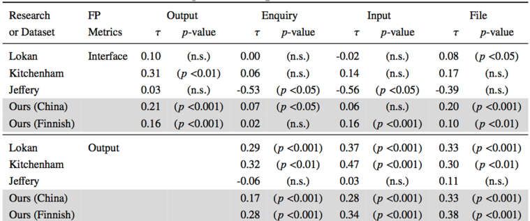
Table 3. Results of Kendall’s t and p-values in previous research and our correlation analysis
4.1.3 Results
The correlation coefficients between FP metrics by our analysis are similar to those in the previous
results by Kitchenham and Känsälä (1993) and Lokan (Lokan, 1999). Table 3 shows the
correlation coefficients between FP metrics for three previous studies and two new results for our
datasets with respect to Kendall’s t B . In our results, Interface shows weak correlation with other
FP metrics ( t B ranges from 0.02 to 0.21). The results of Kitchenham and Känsälä, and Lokan also
show weak correlation with other FP metrics ( t B ranges from -0.02 to 0.31). Output, Enquiry, and
Input show relatively stronger correlation with other FP metrics and it is similar in the results of
Kitchenham and Känsälä, and Lokan. Therefore, we can say that our other correlation coefficients
are very similar to the results by Kitchenham and Känsälä, and Lokan, although our results have
some differences from the results by Kitchenham and Känsälä, and Lokan, where correlations
between FP metrics are statistically significant except the pairs of Interface and Enquiry, and
Interface and Input.
For our datasets, we agree with the results by Kitchenham and Känsälä (1993) and Lokan (Lokan,
1999) on the correlation coefficients between FP metrics. On the other hand, we disagree with the
result by Jeffery and Stathis (1996) on the correlation coefficients.
100International Journal of Mathematical, Engineering and Management Sciences
Vol. 3, No. 2, 90–112, 2018
ISSN: 2455-7749
Fig. 5. Our experiment procedure for RQ2 (focusing on two metrics)
4.2 RQ2: How many bootstrap samples should we use?
4.2.1 Motivation
In our analysis, we adopt BayesLiNGAM, which is an approach for extracting causal-effect
relationships, however, occasionally extracts wrong causal-effect relationships. To overcome this
deficiency, in our previous work (Kondo and Mizuno, 2016), we created 15 new datasets from one
original dataset by conducting 15 times extracting 150 samples by random sampling. We analyzed
the new 15 datasets by BayesLiNGAM, and conducted majority voting to decide which causal-
effect relationship is true. However, there is no evidence to decide the number of new datasets, 15.
To get an evidence for the sufficient number of new datasets, in this paper, we adopt a general
random re-sampling approach, bootstrap sampling (Efron, 1992), to a phase creating new datasets.
This approach provides us a heuristic solution of how many new datasets are sufficient by plotting
distribution and confirming if the distribution is smooth or not.
101International Journal of Mathematical, Engineering and Management Sciences
Vol. 3, No. 2, 90–112, 2018
ISSN: 2455-7749
4.2.2 Approach
Bootstrap sampling is a procedure to estimate a sampling distribution of a model to verify the
model performance in general (Efron, 1992). The sampling distribution is generated by plotting
performances of the model using bootstrap samples. Bootstrap samples are generated by a repeated
method extracting N samples allowing overlapping by random sampling from an original dataset
that has N samples. Bootstrap sampling can be used in outputs of the model are underspecified to
evaluate a performance of the model in general.
Fig. 5 shows the procedure of our experiments that using BayesLiNGAM, extracts causal-effect
relationships. The procedure is as follows:
1. We create two sets (China and Finnish datasets) that consist of M datasets that consist of N
samples. M means the number of bootstrap samples, and N means the sample size of a dataset
(i.e. 499 and 407), respectively.
2. The posterior probabilities of three causal-effect relationships between pairs of metrics are
calculated from the M datasets by BayesLiNGAM for China and Finnish datasets,
respectively.
3. We plot three posterior probabilities of causal-effect relationships using M datasets, and
check the distributions.
Here, we define smoothness of the distribution. We define that a distribution of the causal-effect
relationships is smooth if it satisfies either of the following two conditions under the following
assumption.
Assumption:
We only consider the distribution of the causal-effect relationships that are calculated using
more than a half of bootstrap samples.
Conditions:
Absolute differences of the posterior probabilities (values of x-axis) of the mode and those
of the second mode are less than or equal to 5 and greater than or equal to 50.
Differences of the numbers of the mode entities (values of y-axis) and those of the second
mode entities are greater than or equal to 10.
The assumption aims at removing the distributions of causal-effect relationships that are not
calculated on over a half of bootstrap samples. We suppose such causal-effect relationships might
not true.
The first condition aims at picking up the distributions that have similar posterior probabilities or
different ones between the mode and the second mode. For instance, if the difference of posterior
probabilities between the mode and the second mode are very close (i.e., the difference is less than
or equal to 5), it is reasonable that these values consist of one same distribution and are in a peak
of the same distribution. On the other hand, the probabilities are very far from each other (i.e., the
difference is greater than or equal to 50), it is reasonable that these values have a different
distribution. Otherwise (if the first condition does not hold), the values possibly consist of a
distribution having two peaks (e.g. mixture model).
The second condition considers the value of the y-axis of a distribution. If the value differences of
y-axes between the mode and the second mode are small (i.e., the second condition does not hold),
and the first condition does not hold, it is reasonable that they consist of a distribution having two
102International Journal of Mathematical, Engineering and Management Sciences
Vol. 3, No. 2, 90–112, 2018
ISSN: 2455-7749
peaks. For instance, Fig. 6(c) shows a distribution not smooth, because the posterior probabilities
between the mode and second mode are close and the value difference of y-axes is small.
Here, we need to decide a disturbance density pi (ei ) for BayesLiNGAM. This density is used to
calculate the marginal likelihood for BayesLiNGAM. The density indicates an occurrence
distribution of a disturbance term. We adopt a finite mixture of Gaussian density (MoG) since it
provides better performance than the Gaussian and Laplace distributions (Hoyer and Hyttinen,
2009). As the number of mixtures of MoG, we choose five from our experience (Kondo and
Mizuno, 2016).
We compare two bootstrap sample sizes, 15 and 100. The upper restriction is 100 in our
experiment. Tantithamthavorn et al. (2017) state that 100 is a sufficient value for bootstrap
sampling. Thus, we employ the same upper restriction.
(a) No causal-effect relationship (b) Output is causal to Enquiry (c) Enquiry is causal to Output
Fig. 6. Distributions of posterior probabilities between Output and Enquiry in China dataset when the
number of bootstrap samples is 15
(a) No causal-effect relationship (b) Interface is causal to Enquiry (c) Enquiry is causal to Interface
Fig. 7. Distributions of posterior probabilities between Interface and Enquiry in Finnish dataset when the
number of bootstrap samples is 15
103International Journal of Mathematical, Engineering and Management Sciences
Vol. 3, No. 2, 90–112, 2018
ISSN: 2455-7749
(a) No causal-effect relationship (b) Output is causal to Enquiry (c) Enquiry is causal to Output
Fig. 8. Distributions of posterior probabilities between Output and Enquiry in China dataset when the
number of bootstrap samples is 100
(a) No causal-effect relationship (b) Interface is causal to Enquiry (c) Enquiry is causal to Interface
Fig. 9. Distributions of posterior probabilities between Interface and Enquiry in Finnish dataset when the
number of bootstrap samples is 100
Fig. 10. Our experiment procedure for RQ3 (focusing on two metrics).
104International Journal of Mathematical, Engineering and Management Sciences
Vol. 3, No. 2, 90–112, 2018
ISSN: 2455-7749
4.2.3 Results
As the number of bootstrap samples, 15 is not enough for bootstrap sampling, since the sampling
distribution for bootstrap sampling using 15 samples is not smooth. Figs. 6 and 7 show three
sampling distributions of posterior probabilities where M is 15 for China (between Output and
Enquiry) and Finnish (Interface and Enquiry) datasets. For instance, Fig. 6(c) for “Enquiry is
causal to Output” does not show a smooth sampling distribution.
From our results, the sufficient number of bootstrap samples is 100 to do bootstrap sampling.
When bootstrap sampling uses 100 samples, the sampling distribution is smooth. Figs. 8 and 9
show three sampling distributions of posterior probabilities where M is 100 for China and Finnish
datasets. For instance, Fig. 8(c) for “Enquiry is causal to Output” shows a smooth sampling
distribution.
Figs. 8(b) and 9(b) also do not show a clear distribution. However, posterior probabilities are
distributed to about 0 or 100, and the numbers of datasets in y-axis are similarly between 0 and
100 of posterior probabilities. Thus, it is reasonable to support BayesLiNGAM that cannot identify
this causal-effect relationship into one posterior probability, and shows two types of posterior
probabilities of causal-effect relationships. More details will be discussed in Section 5.1.
As the number of bootstrap samples, 100 is sufficient to do bootstrap sampling. In addition,
BayesLiNGAM cannot decide one posterior probability of the causal-effect relationship in some
cases.
4.3 RQ3: What are causal-effect relationships between FP metrics and Effort?
4.3.1 Motivation
The knowledge of correct causal-effect relationships can contribute to building more accurate
estimation models necessary for software development in the industrial problem. However, so far,
the causal-effect relationships between FP metrics and Effort for effort estimation have not yet
been analyzed.
4.3.2 Approach
To extract causal-effect relationships, we adopt BayesLiNGAM using bootstrap sampling where
the number of bootstrap samples sets to 100 from the answer of RQ2.
Fig. 10 shows the flow of our experiments. The procedure is as follows:
1. We create two sets (Finnish and China datasets) that consist of 100 datasets that consist of N
data. N means the size of a dataset (i.e. 499 and 407), respectively.
2. The 100 causal-effect relationships between pairs of metrics are calculated from the 100
datasets by BayesLiNGAM for China and Finnish datasets, respectively.
3. The causal-effect relationships between pairs of metrics are determined by the majority
voting of the 100 causal-effect relationships. These causal-effect relationships are referred to
as #1. The second-largest ones are referred to as #2.
4. #1 and #2 denote the possibilities of causal-effect relationships
105International Journal of Mathematical, Engineering and Management Sciences
Vol. 3, No. 2, 90–112, 2018
ISSN: 2455-7749
Table 4. Results of upper two causal-effect relationships (mixture: 5) and Kendall’s t and p-values for
China dataset. Upper triangular indicates causal-effect relationships. Lower triangular matrix indicates
correlation coefficients
Table 5. Results of upper two causal-effect relationships (mixture: 5) and Kendall’s t and p-values for
Finnish dataset. Upper triangular indicates causal-effect relationships. Lower triangular matrix indicates
correlation coefficients
4.3.3 Results
Table 4 shows for China dataset, the directions of causal-effect relationships and the number of
datasets which indicate the directions for #1 and #2 in an upper triangular matrix, and the
correlation coefficients in a lower triangular matrix. The symbol “→” means a row metric is causal
to a column metric. The symbol “←” means a column metric is causal to a row metric. “None”
means there is no causal-effect relationship between a row metric and a column metric. The
number in brackets means the number of bootstrap samples. For instance, look at the cells for
Interface and Output in Table 4. None for #1 indicates there is no causal-effect relationship
between Interface and Output. The number in the bracket, 46, indicates this result is calculated
from 46 bootstrap samples. → for #2 indicates Interface is causal to Output. This result is
calculated from 41 bootstrap samples.
In China dataset, when FP metrics and Effort have small correlation coefficients, there are
low possibilities of causal-effect relationships, and when FP metrics and Effort have strong
correlation coefficients, there are high possibilities of causal-effect relationships. Causal-
effect relationships and correlation coefficients have a relationship. For instance, Interface has
small correlation coefficients with other metrics except Effort, and it has low possibilities for a
causal-effect relationship with other metrics except Effort. In addition, Output has a smaller
correlation coefficient with Enquiry than with other metrics, and it also has a low possibility for a
causal-effect relationship with Enquiry.
106International Journal of Mathematical, Engineering and Management Sciences
Vol. 3, No. 2, 90–112, 2018
ISSN: 2455-7749
Table 5 also shows the causal-effect relationships and the correlation coefficients in Finnish
dataset. Finnish dataset has the similar results with China dataset except for Interface and
the pair of Output and File. Causal-effect relationships between Interface and other metrics for
Finnish dataset are different with those for China dataset. For instance, #1 and #2 are different.
Causal-effect relationships between Output and File are also different.
In China dataset, causal-effect relationships are similar to correlation coefficients. On the other
hand, in Finnish dataset, causal-effect relationships are similar to correlation coefficients,
however, some metrics have different directions of causal-effect relationships with China dataset.
Thus, the causal-effect relationships for some metrics possibly depend on datasets.
Table 6. The number of datasets on causal-effect relationships between Interface and Input in Finnish dataset
5. Discussion and Findings
In this section, we give discussions on questions arise from and the findings from the results of
our analysis.
5.1 The sampling distributions for a few causal-effect relationships have two different
distributions by bootstrap sampling using 100 samples.
The sampling distributions by bootstrap sampling sometimes have two different distributions (i.e.
they do not satisfy the first and the second conditions for smooth distributions in Section 4.2.2).
For example, “Output is causal to Enquiry” and “Interface is causal to Enquiry” as shown in Figs.
8 and 9 have two different distributions. Bootstrap sampling typically generates a sampling
distribution, and therefore, these results are unusual.
However, this circumstance does not affect identifying a causal-effect relationship by
BayesLiNGAM based on bootstrap sampling. The pairs of metrics that are involved in such cases
have a clear difference between possibilities of causal-effect relationships. For instance, the
sampling distribution of “Output is causal to Enquiry” in China dataset has two different
distributions. Nevertheless, the sampling distribution of no causal-effect relationship for the pair
of metrics is smooth and has many datasets achieving high posterior probabilities, as in Figs. 8(a)
and 8(b). In addition, the pair of metrics has a high difference between #1 and #2 as shown in
Table 4.
5.2 A few causal-effect relationships have a small difference between #1 and #2.
Identifying a causal-effect relationship is difficult when a difference between #1 and #2 is small
since we could not identify which causal-effect relationships are likelihood in bootstrap sampling.
For instance, the difference between Interface and Output is small both for China and Finnish
107International Journal of Mathematical, Engineering and Management Sciences
Vol. 3, No. 2, 90–112, 2018
ISSN: 2455-7749
datasets. BayesLiNGAM cannot always indicate the correct causal-effect relationships for such
cases. Investigating a further decision method would be useful to support such a case that the
difference between #1 and #2 is small, and thus it is difficult to identify a causal-effect relationship
by BayesLiNGAM.
5.3 BayesLiNGAM sometimes cannot extract a posterior probability for a causal-
effect relationship.
We have conducted bootstrap sampling, however, BayesLiNGAM cannot calculate a posterior
probability for a few datasets (bootstrap samples). Table 6 shows the example of the number of
datasets between Interface and Input in Finnish dataset. BayesLiNGAM successfully calculates
causal-effect relationships for 93 datasets, but fails the calculation for 7 datasets. Nevertheless, we
can identify a causal-effect relationship, since we can get the calculation results for almost all
datasets. In particular, it is more important to identify a causal-effect relationship than to calculate
and identify all posterior probabilities of bootstrap datasets.
5.4 Causal-effect relationships can explain inconsistent results between WC and CC.
Kitchenham et al. (2007) indicate that some studies show inconsistent results on whether there are
differences between WC and CC to estimate effort or not. Our results indicate that causal-effect
relationships are different depending on datasets. The differences of causal-effect relationships
across both WC and CC can lead to such inconsistent results since different causal-effect
relationships have different tendencies. Therefore, the proposed method can be used to analyze
relationships across metrics of WC and CC, and to compare estimation results across WC and CC.
If WC has inconsistent causal-effect relationships like our results, and metrics of CC are also
inconsistency, we can find out one reason why sometimes WC is better than CC, and for other
times, WC is as well as CC. If WC has consistent causal-effect relationships and CC does not have
consistent causal-effect relationships, it indicates that sometimes CC is as well as WC, however,
CC includes worse points than WC does.
5.5 Interface and Output are the best independent explanatory variables for effort
estimation and controlling effort, respectively.
RQ3 is to investigate the directions of causal-effect relationships between FP metrics, and those
in FP metrics and Effort. From results, the causal-effect relationships between FP metrics are
inconsistent, and therefore, it is difficult to discuss general findings. On the other hand, causal-
effect relationships between FP metrics and Effort have consistent results. FP metrics is causal to
Effort metrics in both datasets. Therefore, it is reasonable that every metric can be useful to
estimate effort as an independent explanatory variable. We only consider multicollinearity
problem. From this viewpoint, Interface often has neither the causal-effect relationships nor the
correlation relationships with other FP metrics. Therefore, this is one of the best independent
explanatory variables for effort estimation.
In addition, we can use the interpretation to control effort using FP metrics since FP metrics have
causal-effect relationships for effort. In particular, Output metric is a valuable metric using the
interpretation, since #1 value for Output is high in every dataset.
5.6 How many metrics to which BayesLiNGAM can be applied?
In this paper, using BayesLiNGAM, we only investigate relationships between two metrics of FP
metrics and Effort. BayesLiNGAM can be applied to any number of metrics. However, there is a
108International Journal of Mathematical, Engineering and Management Sciences
Vol. 3, No. 2, 90–112, 2018
ISSN: 2455-7749
computational problem such that the number of DAGs (also the number of combinations of causal-
effect relationships considered) and thus the calculation time increased explosively with the
number of metrics. Indeed, the implementation of BayesLiNGAM used in our experiment shows
us a notification that indicates there are too many inputs if we use over five metrics. To overcome
this problem, Hoyer and Hyttinen (2009) propose an alternative approach, which uses the greedy
search. Hoyer and Hyttinen (2009). report that their approach can be applied to estimate causal-
effect relationships with over six metrics while reducing the calculation time. Investigating causal-
effect relationships among more than two metrics could be an interesting future work.
5.7 How do we decide which correlation relationships or causal-effect relationships
to believe?
In general, causal-effect relationships are better relationships than correlation relationships. This
is because correlation relationships are sometimes spurious correlations as shown in Fig. 1.
Therefore, if there are conflicting results between causal-effect analysis and correlation analysis,
we should confirm whether correlation relationships are not spurious correlations.
6. Threats to Validity
6.1 Construct Validity
We use Kendall’s t for calculating correlation coefficients instead of Pearson correlation
coefficients. Kendall’s t is also adopted in previous studies, and is more powerful to skewed data
and outliers, and our datasets are skewed and have many outliers. Thus, it is valid to adopt
Kendall’s t to calculate correlation coefficients.
For using BayesLiNGAM, we assume that the disturbance density is a finite mixture of Gaussian
density and the number of mixture is five. That means that we approximate population of data as
a five mixture of Gaussian density.
For experimental analysis, we use two datasets, China and Finnish datasets, which have been
adopted previous studies on effort estimation (Sigweni et al., 2016; Bettenburg et al., 2012). Thus,
it is valid to use these datasets.
6.2 External Validity
Correlation coefficients between FP metrics already have been investigated in previous studies,
and our results are similar to the majority of previous results. Therefore, results of correlation
coefficients are general.
Results of causal-effect relationships are also general since we adopt two types of datasets, and
adopt bootstrap sampling. Bootstrap sampling supports providing a general result.
6.3 Reliability
We use BayesLiNGAM (open at https://www.cs.helsinki.fi/group/neuroinf/lingam/bayeslingam/)
that was implemented by Hoyer and Hyttinen who originally proposed BayesLiNGAM. Thus,
reliability of results of BayesLiNGAM is high.
In addition, we provide all data and scripts that are used for our study at https://se.is.kit.ac.jp/~m-
kondo/BayesLiNGAM.tar.bz2. Thus, anyone can easily conduct and confirm our analysis.
109International Journal of Mathematical, Engineering and Management Sciences
Vol. 3, No. 2, 90–112, 2018
ISSN: 2455-7749
7. Conclusion
In this paper, we presented a causal-effect analysis between FP metrics and effort using
BayesLiNGAM. Using the proposed analysis, we can investigate the directions of causal-effect
relationships among the metrics. Therefore, our analysis can support building a good effort
estimation model.
From the results of our analysis using two datasets, we confirmed that causal-effect relationships
between FP metrics are similar to correlation relationships between them, and most of causal-
effect relationships have same directions. However, a few causal-effect relationships have
different directions in difference datasets.
We also confirmed that when FP metrics and effort have a correlation, they also have causal-effect
relationships. Thus, correlations between FP metrics and effort are not spurious correlations.
In addition, from our results, Interface, one of the mostly used FP metrics, does not have strong
correlation coefficients and causal-effect relationships with other FP metrics. This result indicates
that Interface is the best FP metric to build an effort estimation model since it then does not cause
a multicollinearity problem.
Our future work includes extracting new features from original features (e.g. metrics) to solve the
multicollinearity problem. We could make the new features that can overcome the
multicollinearity problem by integrating correlated features. Although a stepwise regression
approach (Mendes and Mosley, 2001) is already proposed to remove correlated features, we plan
to make the new features that contribute to the performance improvement of an objective task. In
particular, we are interested in adopting a neural network approach.
References
Abran, A., Silva, I., & Primera, L. (2002). Field studies using functional size measurement in building
estimation models for software maintenance. Journal of Software Maintenance and Evolution:
Research and Practice, 14(1), 31–64.
Ahn, Y., Suh, J., Kim, S., & Kim, H. (2003). The software maintenance project effort estimation model
based on function points. Journal of Software Maintenance and Evolution: Research and Practice,
15(2), 71–85.
Albrecht, A. J., & Gaffney, J. E. (1983). Software function, source lines of code, and development effort
prediction: a software science validation. IEEE Transactions on Software Engineering, SE-9, (6), 639–
648.
Bettenburg, N., Nagappan, M., & Hassan, A. E. (2012). Think locally, act globally: Improving defect and
effort prediction models. In Proceedings of the 9th IEEE Working Conference on Mining Software
Repositories (MSR) (pp. 60–69).
Briand, L. C., El Emam, K., Surmann, D., Wieczorek, I., & Maxwell, K. D. (1999). An assessment and
comparison of common software cost estimation modeling techniques. In Proceedings of the 1999
International Conference on Software Engineering (ICSE) (pp. 313–323).
Efron, B. (1992). Bootstrap methods: another look at the jackknife. In Breakthroughs in Statistics (pp. 569–
593). Springer.
110International Journal of Mathematical, Engineering and Management Sciences
Vol. 3, No. 2, 90–112, 2018
ISSN: 2455-7749
Farrar, D. E., & Glauber, R. R. (1967). Multicollinearity in regression analysis: the problem revisited. The
Review of Economics and Statistics, 49(1), 92-107.
Green, M. J., Leyland, A. H., Sweeting, H., & Benzeval, M. (2017). Causal effects of transitions to adult
roles on early adult smoking and drinking: Evidence from three cohorts. Social Science & Medicine,
187, 193-202
Heinze-Deml, C., Maathuis, M. H., & Meinshausen, N. (2017). Causal structure learning. arXiv preprint
arXiv:1706.09141.
Hernán, M. A. (2004). A definition of causal effect for epidemiological research. Journal of Epidemiology
& Community Health, 58(4), 265-271.
Holland, P. W., Glymour, C., & Granger, C. (1985). Statistics and causal inference. ETS Research Report
Series, 1985(2), 1-72.
Hoyer, P. O., & Hyttinen, A. (2009). Bayesian discovery of linear acyclic causal models. In Proceedings of
the 25th Conference on Uncertainty in Artificial Intelligence (pp. 240–248). AUAI Press.
Jeffery, R., & Stathis, J. (1996). Function point sizing: structure, validity and applicability. Empirical Software
Engineering, 1(1), 11–30.
Jeffery, R., Ruhe, M., & Wieczorek, I. (2000). A comparative study of two software development cost
modeling techniques using multi-organizational and company-specific data. Information and Software
Technology, 42(14), 1009 - 1016.
Jorgensen, M., & Shepperd, M. (2007). A systematic review of software development cost estimation studies.
IEEE Transactions on Software Engineering, 33(1), 33-53.
Kitchenham, B. A., Mendes, E., & Travassos, G. H. (2007, May). Cross versus within-company cost
estimation studies: A systematic review. IEEE Transactions on Software Engineering, 33(5), 316-329.
Kitchenham, B., & Känsälä, K. (1993). Inter-item correlations among function points. In Proceedings of the
15th International Conference on Software Engineering (ICSE) (pp. 477–480).
Kleinberg, S., & Hripcsak, G. (2011). A review of causal inference for biomedical informatics. Journal of
Biomedical Informatics, 44(6), 1102-1112.
Kondo, M., & Mizuno, O. (2016). Analysis on causal-effect relationship in effort metrics using Bayesian
LiNGAM. In Proceedings of 2016 IEEE International Symposium on Software Reliability Engineering
Workshops (ISSREW) (pp. 47–48).
Lokan, C. J. (1999). An empirical study of the correlations between function point elements [software
metrics]. In Proceedings of 1999 6th International Software Metrics Symposium (pp. 200–206).
Mendes, E., & Mosley, N. (2001). Comparing effort prediction models for web design and authoring using
boxplots. In Proceedings of the 24th Australasian Computer Science Conference (ACSC) (pp. 125–
133).
Mendes, E., Lokan, C., Harrison, R., & Triggs, C. (2005). A replicated comparison of cross-company and
within-company effort estimation models using the ISBSG database. In Proceedings of the 11th IEEE
International Symposium Software Metrics (pp. 10).
Menzies, T., Krishna, R., & Pryor, D. (2016). The promise repository of empirical software engineering
data; http://openscience.us/repo. North Carolina State University.
Messerli, F. H. (2012). Chocolate consumption, cognitive function, and Nobel laureates. The New England
Journal of Medicine, 367(16), 1562.
111International Journal of Mathematical, Engineering and Management Sciences
Vol. 3, No. 2, 90–112, 2018
ISSN: 2455-7749
Molokken, K., & Jorgensen, M. (2003). A review of software surveys on software effort estimation. In
Proceedings of 2003 International Symposium on Empirical Software Engineering (ISESE) (pp. 223–
230).
Pearl, J. (2002). Causality: models, reasoning, and inference. IIE Transactions, 34(6), 583–589.
Pfister, N., Bühlmann, P., & Peters, J. (2017). Invariant causal prediction for sequential data. arXiv preprint
arXiv:1706.08058.
Robins, J. (1986). A new approach to causal inference in mortality studies with a sustained exposure
period—application to control of the healthy worker survivor effect. Mathematical Modelling, 7(9-12),
1393-1512.
Shimizu, S., Hoyer, P. O., Hyvärinen, A., & Kerminen, A. (2006). A linear non-Gaussian acyclic model for
causal discovery. Journal of Machine Learning Research, 7, 2003–2030.
Sigweni, B., Shepperd, M., & Forselius, P. (2015, 3). Finnish software effort dataset (Online),
https://figshare.com/articles/Finnish_Effort_Estimation_Dataset/1334271, (accessed: 2017-7-30).
Sigweni, B., Shepperd, M., & Turchi, T. (2016). Realistic assessment of software effort estimation models.
In Proceedings of the 20th International Conference on Evaluation and Assessment in Software
Engineering (p. 41).
Sprent, P., & Smeeton, N. C. (2016). Applied nonparametric statistical methods. CRC Press.
Takagi, Y., Mizuno, O., & Kikuno, T. (2005). An empirical approach to characterizing risky software projects
based on logistic regression analysis. Empirical Software Engineering, 10(4), 495-515.
Tantithamthavorn, C., McIntosh, S., Hassan, A. E., & Matsumoto, K. (2017). An empirical comparison of
model validation techniques for defect prediction models. IEEE Transactions on Software Engineering,
43(1), 1-18.
The Standish Group (1994). Chaos. Technical report, The Standish Group International Inc.
Uzzafer, M. (2016). Bootstrap correlation analysis of function point elements. International Journal of
Database Theory and Application, 9(3), 11–18.
Wen, J., Li, S., Lin, Z., Hu, Y., & Huang, C. (2012). Systematic literature review of machine learning based
software development effort estimation models. Information and Software Technology, 54(1), 41–59.
You, C. (2016). R tutorial (Online), http://www.r-tutor.com/elementary-statistics/numerical-
measures/skewness, (accessed 2017-7-16).
112You can also read