GNSS Meteorology for Disastrous Rainfalls in 2017-2019 Summer in SW Japan: A New Approach Utilizing Atmospheric Delay Gradients - Frontiers
←
→
Page content transcription
If your browser does not render page correctly, please read the page content below
ORIGINAL RESEARCH
                                                                                                                                              published: 23 June 2020
                                                                                                                                        doi: 10.3389/feart.2020.00182

                                             GNSS Meteorology for Disastrous
                                             Rainfalls in 2017–2019 Summer in SW
                                             Japan: A New Approach Utilizing
                                             Atmospheric Delay Gradients
                                             Syachrul Arief 1,2* and Kosuke Heki 1
                                             1
                                               Department of Natural History Sciences, Hokkaido University, Sapporo, Japan, 2 Geospatial Information Agency, Cibinong,
                                             Indonesia

                                             We studied disastrous heavy rainfall episodes in 2017–2019 summer in SW Japan,
                                             especially in the Kyushu region using tropospheric delay data from the Japanese dense
                                             global navigation satellite system (GNSS) network GEONET (GNSS Earth Observation
                                             Network). This region often suffers from extremely heavy rains associated with stationary
                                             fronts during summer. In this study, we first analyze behaviors of water vapor on July 6,
                                             2018, using tropospheric parameters obtained from the database at the University of
                              Edited by:
                          Giovanni Nico,     Nevada, Reno. The data set includes tropospheric delay gradient vectors (G), as well
 Istituto per le Applicazioni del Calcolo    as zenith tropospheric delays (ZTD), estimated every 5 min. At first, we interpolated G
             “Mauro Picone” (IAC), Italy
                                             to obtain those at grid points and calculated their convergence, similar to the quantity
                        Reviewed by:
             Bijoy Vengasseril Thampi,
                                             proposed by Shoji (2013) as water vapor concentration (WVC) index. We obtained zenith
   Science Systems and Applications,         wet delay (ZWD) from ZTD by removing zenith hydrostatic delay. The raw ZWD values
                    Inc., United States
                                             do not really reflect the wetness of the atmosphere above the GNSS station because
                           Daoyi Gong,
      Beijing Normal University, China       they largely depend on the station altitudes. To study the dynamics of water vapor
                  *Correspondence:           before heavy rains, we estimated ZWD converted to the values at sea level. In the
                        Syachrul Arief       inversion scheme, we used G at all GEONET stations and ZWD data at low-altitude
            syachrul@eis.hokudai.ac.jp
                                             (50 mm/h) episodes occurred, that is, July 5, 2017, July
           Published: 23 June 2020
                                             6, 2018, and August 27, 2019. Next, we performed high time resolution analysis (every
                             Citation:
      Arief S and Heki K (2020) GNSS         5 min) on the days of heavy rain. The results suggest that both WVC and sea-level ZWD
   Meteorology for Disastrous Rainfalls      go up prior to the onset of the rain, and ZWD decreases rapidly once the heavy rain
 in 2017–2019 Summer in SW Japan:
             A New Approach Utilizing
                                             started. It is a future issue, however, how far these two quantities contribute to forecast
        Atmospheric Delay Gradients.         heavy rains.
               Front. Earth Sci. 8:182.
       doi: 10.3389/feart.2020.00182         Keywords: heavy rain, GNSS, Japan, tropospheric gradient, water vapor convergence, zenith wet delay

Frontiers in Earth Science | www.frontiersin.org                                   1                                                 June 2020 | Volume 8 | Article 182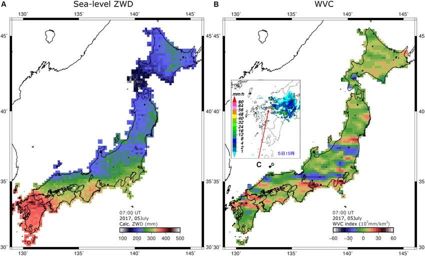
Arief and Heki                                                                                  GNSS-Meteorology, PWV, Gradient, Japan, Heavy Rain

INTRODUCTION                                                              try to reconstruct ZWD in inland regions (especially in high-
                                                                          altitude regions) by spatially integrating G.
Disastrous heavy rains in summer 2017 to 2019 in SW Japan                     The purpose of this study is to show the implication of
caused a lot of damage to property and human lives. The                   utilizing tropospheric delay gradients, in addition to ZWD, to
Japan Meteorological Agency (JMA) officially named the extreme            improve our understanding of water vapor dynamics during
rainfall event in 2018 July as “The Heavy Rain Event of July 2018.”       heavy rains. For this purpose, we reconstruct ZWD and calculate
Precipitation records at meteorological stations show extreme             WVC and compare them with in situ rainfall data from AMEDAS
rainfalls from June 28 to July 8, 2018, especially in the northern        (Automated Meteorological Data Acquisition System) stations of
part of the Kyushu District. Figure 1 shows the precipitation             JMA. Finally, we study the behaviors of these quantities common
rate in the high-resolution nowcast rainfall map at 17:00 JST             for the three heavy rain cases in SW Japan in summer 2017–2019.
(08:00 UT), July 6, 2018, from JMA. This was obtained by
a weather radar with a 250-m resolution every 5 min. Such
meteorological radars have been operated by JMA at 20 stations            DATA AND METHODS: CASE STUDY
throughout Japan. The heavy rain occurred over a patchy region            FOR THE 2018 HEAVY RAIN
elongated in NE-SW and overlap with the stationary front. Water
vapor transported along the front from SW is thought to have              We use the data from the dense GNSS network GEONET for the
caused the heavy rain.                                                    entire country operated by the Geospatial Information Authority
   The concept of ground-based global navigation satellite                (Tsuji and Hatanaka, 2018). It consists of more than 1,300
system (GNSS) meteorology was proposed initially by Bevis et al.          continuously observing stations in Japan with a typical separation
(1992), and meteorological utilization of the Japanese GEONET             distance of 15 to 30 km. Because its official solution (F3 solution)
has been sought (e.g., Tsuda et al., 1998). Nowadays, GNSS                does not include tropospheric parameters in high temporal
meteorology has become one of the essential means to observe              resolution (Nakagawa et al., 2009), we used tropospheric delay
precipitable water vapor (PWV), and PWV data from GEONET                  data from the UNR database (Blewitt et al., 2018). They estimated
have been assimilated in the mesoscale model of JMA to improve            tropospheric parameters using the GIPSY/OASIS-II version 6.1.1
weather forecast accuracy since 2009 (e.g., Shoji, 2015). In this         software with the Precise Point Positioning technique (Zumberge
study, we apply a new method of GNSS meteorology to utilize               et al., 1997) using the products for satellite orbits and clocks from
atmospheric delay gradients, reflecting azimuthal asymmetry of            Jet Propulsion Laboratory. They employ the elevation cutoff angle
water vapor (MacMillan, 1995), for the 2017–2019 heavy rain               of 7◦ and estimate ZTD and the atmospheric delay gradients
cases in SW Japan.                                                        every 5 min (Vaclavovic and Dousa, 2015). They follow the 2010
   Miyazaki et al. (2003) focused on such atmospheric delay               IERS convention (Petit and Luzum, 2010), and used the Global
gradients and showed that the temporal and spatial variations of          Mapping Function (Böhm et al., 2006), and troposphere gradient
the gradients were compatible with the humidity fields derived            model of Chen and Herring (1997).
from zenith wet delay (ZWD) and with the meteorological
conditions in 1996 summer over the Japanese Islands (especially           ZWD and Tropospheric Delay Gradients
during a front passages). Shoji (2013) and Brenot et al.                  The equation below is formulated by MacMillan (1995) and
(2013) demonstrated the important role of the atmospheric                 explains that the slant path delay (SPD) at the elevation angle θ
delay gradients to detect smaller scale structures of the                 and the azimuth angle ϕ measured clockwise from north can be
troposphere than ZWD.                                                     expressed as follows.
   Recently, Zus et al. (2019) have successfully processed
the Central Europe GNSS network data to show that the                       SPD(θ, φ) = m(θ) · [ZTD + cotθ(Gn cosφ + Ge sinφ)] + ε (1)
interpolation of ZWD observed with a sparse network can
be improved by utilizing tropospheric delay gradients. They               There, m(θ) is the isotropic mapping function that shows the
showed significant accuracy improvement for the simulation of             ratio of SPD to ZTD, and Gn and Ge are the north and east
the numerical weather model, and for the agreement of the                 components, respectively, of the tropospheric delay gradient
simulation results with real observations, relative to the cases          vectors G, and ε is the modeling error. ZTD is the refractivity of
without utilizing tropospheric delay gradients.                           the atmosphere integrated in the vertical direction and is the sum
   In this study, we propose a new method to use tropospheric             of zenith hydrostatic delay (ZHD) and ZWD. In this study, we
delay gradients to study heavy rain phenomena in Japan using              calculated surface pressure at the GNSS stations assuming 1 atm
the data from the GEONET data. At first, we analyze behaviors             at the sea level. Then, we calculated ZHD and subtracted it from
of water vapor on July 6, 2018, using tropospheric parameters             ZTD to isolate ZWD. Considering average variability of surface
obtained from the database at the University of Nevada, Reno              pressure, errors by this approximation for summer ZWD remain
(UNR; Blewitt et al., 2018). The data set includes tropospheric           within a few percent.
delay gradient vectors (G), as well as zenith tropospheric delays             Tropospheric delay gradients are also the sum of hydrostatic
(ZTDs), estimated every 5 min. We interpolate G to obtain those           and wet contributions. Because we analyze summer data, we
at grid points and calculated their convergence, similar to the           assumed that the latter is dominant and used the gradient as
index proposed by Shoji (2013) as water vapor concentration               those representing the water vapor. Because of the low scale
(WVC). Then, taking advantage of the dense GNSS network, we               height of water vapor (∼2.5 km), ZWD highly depends on the

Frontiers in Earth Science | www.frontiersin.org                      2                                           June 2020 | Volume 8 | Article 182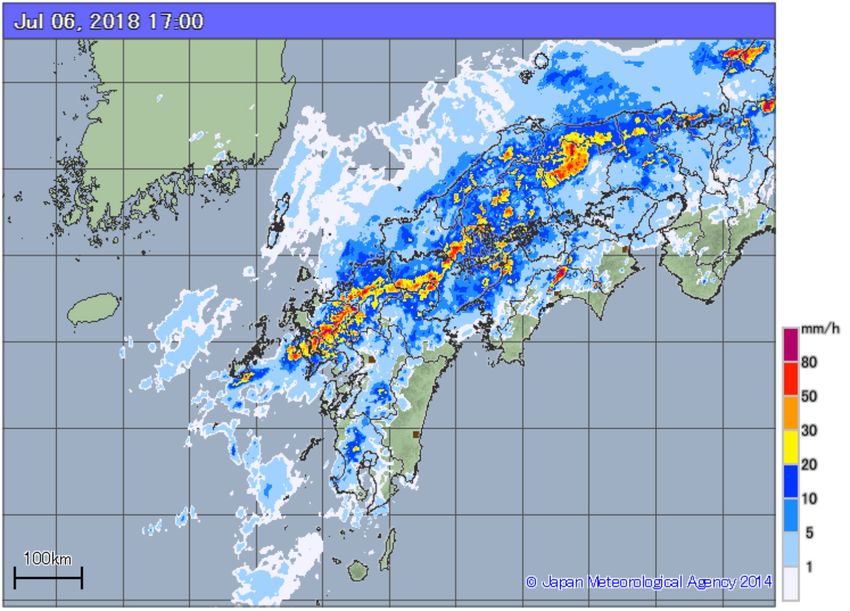
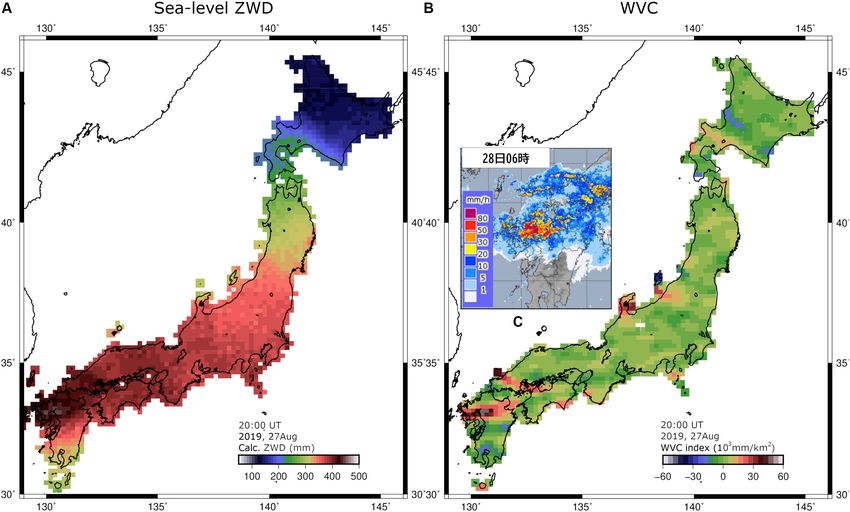
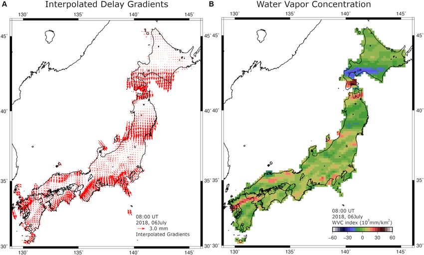
Arief and Heki                                                                                                  GNSS-Meteorology, PWV, Gradient, Japan, Heavy Rain

  FIGURE 1 | High-resolution map of the rainfall rate at 17:00 JST (08:00 UT) July 6, 2018, from JMA (https://www.data.jma.go.jp/fcd/yoho/meshjirei/jirei01/high
  resorad/index.html).

  FIGURE 2 | (A) Atmospheric delay gradients at grid points at 17 JST (08 UT) on July 6, 2018 (raw gradient data are shown in Figure 4A). Using these gradient
  vectors at grid points, we calculated their convergence shown in (B), similar to WVC index defined by Shoji (2013).

Frontiers in Earth Science | www.frontiersin.org                                   3                                                 June 2020 | Volume 8 | Article 182
Arief and Heki GNSS-Meteorology, PWV, Gradient, Japan, Heavy Rain
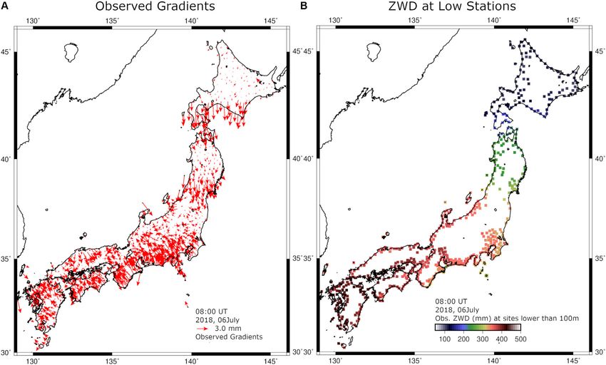
station altitude; that is, small ZWD observed at highland does not As the first case study, we investigate water vapor in the heavy
always imply low humidity of the troposphere above that station. rainfall episode at 08 UT (17 JST) July 6, 2018. There are strong
On the other hand, atmospheric delay gradients are observed by southward gradients in southern Hokkaido and central Tohoku,
directly comparing atmospheric delays in different azimuths and suggesting southwestward increase of water vapor. In northern
hardly suffer from the station altitude (Shoji, 2013). This is the Kyushu, we can see large gradient vectors line up, suggesting high
reason why we use troposphere gradients to reconstruct ZWD concentration of water vapor there.
converted to sea level.
Sea-Level ZWD
Water Vapor Concentration In our study, in addition to WVC, we also reconstruct sea-
Shoji (2013) suggested that two new quantities, WVC and level ZWD using the observed tropospheric delay gradients and
WVI (water vapor inhomogeneity) indices, provide valuable ZWD at low elevation (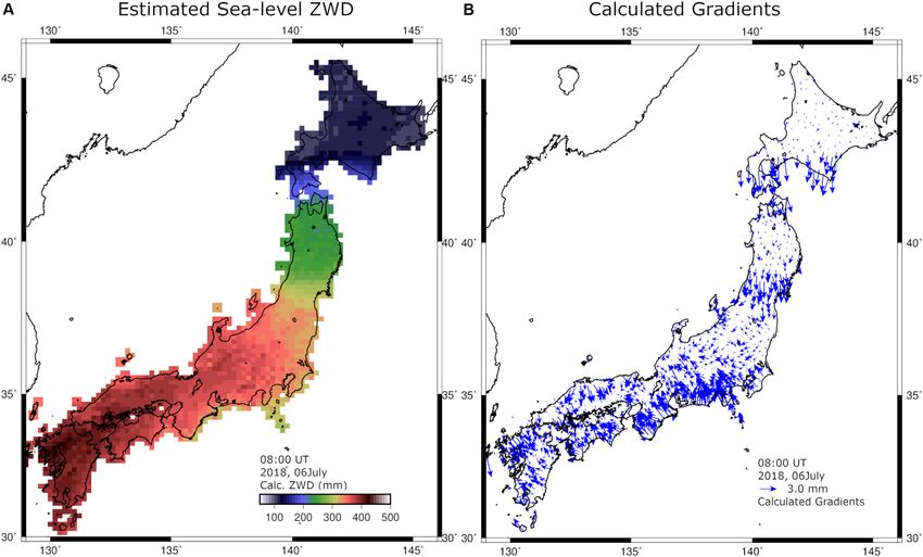
Arief and Heki                                                                                                   GNSS-Meteorology, PWV, Gradient, Japan, Heavy Rain

  FIGURE 4 | Input data for the inversion of sea-level ZWD at 17 JST (08 UT) on July 6, 2018. (A) shows the tropospheric delay gradients at all the GEONET stations,
  and (B) is the ZWD at stations with elevations
Arief and Heki                                                                                             GNSS-Meteorology, PWV, Gradient, Japan, Heavy Rain

  FIGURE 6 | Estimated sea-level ZWD (A) and WVC (B) at 07 UT (16 JST) on July 5, 2017. (C) shows the rain rate map from Japan Meteorology Agency [JMA]
  (2017) at the epoch 1 h earlier (06 UT) than (A,B).

  FIGURE 7 | Estimated sea-level ZWD (A) and WVC index (B) at 20 UT (05 JST) on August 27 (August 28 in JST), 2019. (C) shows the rain rate map from Japan
  Meteorological Agency [JMA] (2019) at the epoch 1 h later (21UT) than (A,B).

Frontiers in Earth Science | www.frontiersin.org                               6                                              June 2020 | Volume 8 | Article 182
Arief and Heki GNSS-Meteorology, PWV, Gradient, Japan, Heavy Rain
To regularize the inversion, we constrain the sea-level ZWD at number of observations is twice as large as the number of GNSS
the grids closest to the GNSS stations with altitude less than 100 m stations, ∼2,600. The number of GNSS stations with altitudes of
to the observed ZWD. They indicate that the sea-level ZWD at less than 100 m is ∼100. In Figures 4, 5, we show inputs and
the grid point x(i, j) is the same as the ZWD y(k) observed at the outputs of the inversion, respectively. In Figure 5B, we confirm
k’th GNSS station, that is, that the atmospheric delay gradient vectors at GNSS stations
calculated using the estimated distribution of sea-level ZWD.
x i, j = y k . (6)
They are similar to the input shown in Figure 4A, suggesting
We then performed inversion also applying a continuity that the inversion is successful. The root-mean-square error
constraint. When we estimate the sea-level ZWD over the entire between the observed and calculated atmospheric delay gradient
Japanese Islands, the number of parameters is ∼1,600, and the is ∼0.65 mm in this case.
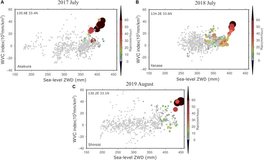
FIGURE 8 | Distribution of hourly values of WVC (vertical axis), sea-level ZWD (horizontal axis), and hourly rain rate (color and circle size) for July 2017 (A), July 2018
(B), and August 2019 (C). The rain rate was measured at the Asakura, Yanase, and Shiroishi AMEDAS stations, respectively, and WVC and ZWD are the values at
their nearest grid points (coordinates given at the upper left corners).
FIGURE 9 | Same as Figures 8B,C, but we stacked data for 12 and 5 AMEDAS stations showing hourly rain rate exceeding 50 mm in July 2018 (A) and August
2019 (B), respectively. Again, we compare hourly rain rates with the WVC and ZWD, calculated at the nearest grid points of the AMEDAS stations.
Frontiers in Earth Science | www.frontiersin.org 7 June 2020 | Volume 8 | Article 182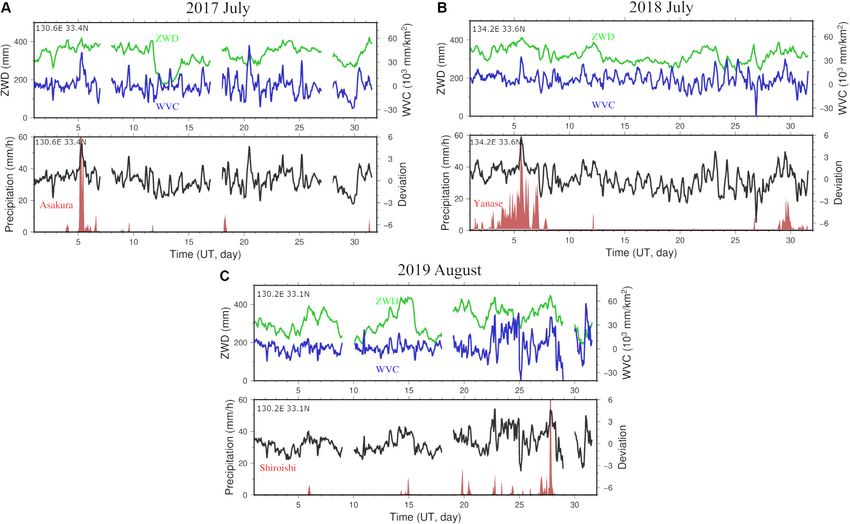
Arief and Heki                                                                                               GNSS-Meteorology, PWV, Gradient, Japan, Heavy Rain

RESULTS AND DISCUSSION                                                                 Here we perform the same calculation for a heavy rain episode
                                                                                    on July 5, 2017, at 07 UT (16 JST) and show the results in Figure 6.
Figure 5A shows high ZWD throughout SW Japan, but such                              These figures also show, like in the 2018 case, that both the sea-
a ZWD map still lacks spatial resolution to pinpoint heavy                          level ZWD and WVC are high where it rains heavily as shown in
rain as indicated in Figure 1. At a glance, WVC in Figure 2B                        Japan Meteorology Agency [JMA] (2017).
shows good coincidence with the heavy rain given in red                                Likewise, Figure 7 shows the sea-level ZWD and WVC for
and orange colors in Figure 1. However, there are regions                           a heavy rainfall episode in August 2019. WVC index pinpoints
where WVC is high but heavy rain does not occur. This                               heavy rainfall, consistent with the information compiled by Japan
suggests that both two quantities need to be high for the                           Meteorological Agency [JMA] (2019).
occurrence of heavy rains. In this section, we study long- and                         From these results, we hypothesize that heavy rainfall occurs
short-term behaviors of the two quantities in several recent                        when both the ZWD and WVC are high. Next, we try
heavy rain episodes in SW Japan. For the former, we see                             to test the hypothesis by studying time series of the two
hourly changes of WVC and sea-level ZWD over 1-month                                quantities and rain rate.
periods including the heavy rain episodes. For the latter, we
study the change of these quantities every 5 min over the
days of heavy rain.
                                                                                    WVC, Sea-Level ZWD, and Heavy Rain
                                                                                    Here we try to justify our working hypothesis that heavy rains
                                                                                    occur when the WVC index and sea-level ZWD are both high
The 2017 and 2019 Heavy Rain Cases                                                  by analyzing the distribution of water vapor every hour in the
In Figures 2B, 5B, we show the WVC index and sea-level ZWD                          three cases, July 2017, July 2018, and August 2019. We present
at 08.00 UT (17 JST) when heavy rain occurred. This can be                          the results in Figure 8, which explains the scatter plot of sea-level
compared with the rain images from the JMA, as shown in                             ZWD and WVC, along with hourly rainfall data based on
Figure 1. By comparing Figures 1, 2B, we can see that the WVC                       observations at the AMEDAS station of JMA.
index successfully pinpoints the heavy rain. This is also consistent                   We selected the AMEDAS station showing the largest rain
with the detailed report of this heavy rain episode compiled by                     for the three episodes, that is, the Asakura station for 2017, the
Japan Meteorology Agency [JMA] (2018).                                              Yanase station for 2018, and the Shiroishi station for 2019. These

  FIGURE 10 | Time series of the two quantities shown in Figure 8, WVC and sea level ZWD (blue and green in the top panels), and rain rate at the nearest AMEDAS
  stations (red in the bottom panels). The bottom panels also show a new quantity (labeled as “Deviation”) in black, the sum of the standard deviation of the two
  quantities. They are for July 2017 (A), July 2018 (B), and August 2019 (C). High hourly rain rates occur when both the WVC and ZWD record very high values.

Frontiers in Earth Science | www.frontiersin.org                                8                                                June 2020 | Volume 8 | Article 182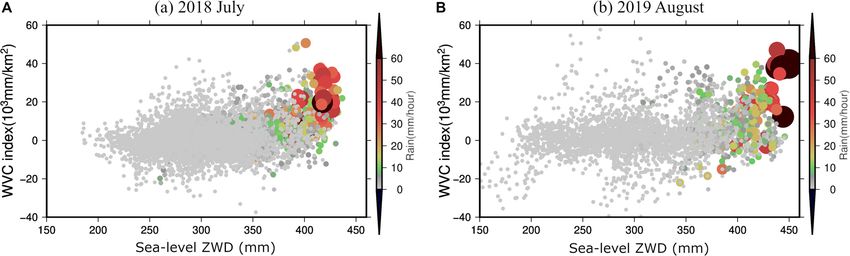
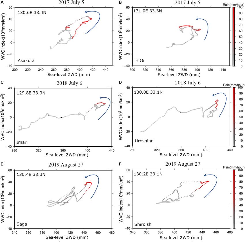
Arief and Heki                                                                                                   GNSS-Meteorology, PWV, Gradient, Japan, Heavy Rain

three stations are all located in northern Kyushu and recorded                          and found 12 stations for the 2018 July and 5 stations for the
heavy rains exceeding 50 mm/h. Then we picked up the grid                               2019 August, the months including heavy rain episodes. The 2017
point closest to these AMEDAS and compare the three quantities                          heavy rain was quite local (limited to northern Kyushu); we could
over a month, that is, July 2017, July 2018, and August 2019.                           not find enough number of AMEDAS stations showing rains
We can see that ZWD values are high up to 400 mm, and WVC                               exceeding 50 mm/h. From Figure 9A, we find that the probability
index goes up to 40 × 103 mm/km2 when heavy rain exceeding                              of the heavy rain (>50 mm/h) was 14% for the range of ZWD
50 mm/h occurred on July 5, 2017, July 6, 2018, and August 27,                          (400–450 mm) and WVC index (35–50 × 103 mm/km2 ), for July
2019 (Figure 8).                                                                        2018. Likewise, for August 2019, the heavy rain occurred 50%
   Next, we look for data from more AMEDAS stations in Japan                            for the same range of ZWD and WVC index. If we count rains
on the same days showing hourly rain rates exceeding 50 mm/h                            exceeding 20 mm/h, then the percentages go up to 71% for July

  FIGURE 11 | High time resolution (5-min resolution) behaviors of rain rate in the sea-level ZWD-WVC space during the heavy rain days, July 5, 2017 (A: Asakura, B:
  Hita), July 6, 2018 (C: Imari, D: Ureshino), and August 27, 2019 (E: Saga, F: Shiroishi). The color indicates hourly precipitation of AMEDAS stations interpolated to
  match the time resolution of sea-level ZWD and WVC.

Frontiers in Earth Science | www.frontiersin.org                                    9                                                  June 2020 | Volume 8 | Article 182
Arief and Heki                                                                                                      GNSS-Meteorology, PWV, Gradient, Japan, Heavy Rain

2018 and 78% for August 2019. These results indicate that both                             showed the importance of the WVC index reflecting small-scale
the WVC index and sea-level ZWD are high when heavy rains                                  enhancement of water vapor. As seen in the scatter diagrams in
occur. The results also suggest that heavy rains may not occur                             Figures 8, 9, sea-level ZWD and WVC are not correlated; that
even when these two quantities are high. Next, we will show time                           is, high sea-level ZWD does not always mean high WVC and
series of these quantities.                                                                vice versa. We showed that heavy rain occurs only when both
                                                                                           quantities show high values.
Time-Series Analysis                                                                           The results suggest that monitoring these quantities is useful
In Figure 10, we plot the quantities in Figure 8 as the functions                          for the nowcast of heavy rains. However, their potential to
of time. The two quantities WVC and sea-level ZWD are given                                forecast heavy rains is yet to be studied. As the next step, we will
at the top, whereas the rain rate is given at the bottom. The                              need to explore the way to use these two quantities for weather
bottom panels also include the time series labeled as “deviation.”                         forecast, for example, by putting them to numerical weather
This quantity indicates the sum of the deviations of WVC and                               models by some means. Computation time of sea-level ZWD and
sea-level ZWD from their averages normalized by their standard                             WVC is short, and we can convert ZTD values estimated by GNSS
deviations. For example, if both quantities deviate from the                               data analysis in near real time to sea-level ZWD and WVC.
means by 2σ, the deviation is 4.
    Figure 10 clearly shows that the two quantities show large
deviations from the average values whenever heavy rains occur.                             DATA AVAILABILITY STATEMENT
We also see sometimes that high deviation does not coincide
                                                                                           The datasets generated for this study are available on request to
with a heavy rain, for example, July 20, 2017, and July 23, 2018.
                                                                                           the corresponding author. Tropospheric parameters used in this
Regarding the time sequence, the high WVC/ZWD times seem to
                                                                                           study are available from geodesy.unr.edu.
“coincide” with heavy rains rather than “precede” them. Hence,
the usefulness of monitoring these quantities for weather forecast
is not clear from this figure.
    Lastly, we analyzed high time resolution (every 5 min)
                                                                                           AUTHOR CONTRIBUTIONS
behaviors of WVC, ZWD, and rain rate, for the three heavy                                  All authors listed have made a substantial, direct and intellectual
rain days in July 5, 2017, July 6, 2018, and August 27, 2019,                              contribution to the work, and approved it for publication.
selecting two AMEDAS stations from each episode (Figure 11).
We estimated the sea-level ZWD and WVC every 5 min for these
3 days. The results show that both WVC indices and sea-level                               FUNDING
ZWD show large values at the start of the heavy rains. However,
for many cases (e.g., Figures 11A,E,F), heavy rains already started                        This research was funded by the Ministry of Research,
before the two quantities reach their peaks, suggesting limited                            Technology, and Higher Education (Kemenristekdikti),
applicability of these quantities for weather forecast. ZWD often                          Indonesia, in collaboration with the World Bank conducting
showed rapid declines after the start of the heavy rainfalls possibly                      Research and Innovation in Science and Technology Project
because of the transformation of water vapor to liquid water.                              (RISET-Pro) through Loan No. 8245-ID.

CONCLUSION                                                                                 ACKNOWLEDGMENTS
The atmospheric delay gradients are little influenced by station                           We thank RISET-Pro Kemenristekdikti, and Nevada Geodetic
altitudes and provide useful information of spatial gradient of                            Laboratory (NGL) – University of Nevada, Reno, for
relative humidity in lower atmosphere. By using atmospheric                                providing tropospheric parameters for worldwide GNSS
delay gradients, we could estimate distributions of sea-level                              stations (ftp://gneiss.nbmg.unr.edu/). We also thank Japan
ZWD, reflecting relative humidity of the air column above                                  Meteorological Agency (JMA) for operating Automated
the station. This is possible only in regions with dense GNSS                              Meteorological Data Acquisition System (AMeDAS) stations.
networks like Japan, because we relate tropospheric delay                                  We thank Yoshinori Shoji, MRI, for useful discussions, and two
gradient to horizontal spatial gradient of ZWD. We also                                    referees for constructive comments.

REFERENCES                                                                                 Böhm, J., Niell, A., Tregoning, P., and Schuh, H. (2006). Global
                                                                                              Mapping Function (GMF): a new empirical mapping function based
Bevis, M., Businger, S., Herring, T. A., Rocken, C., Anthes, R. A., and Ware, R. H.           on numerical weather model data. 33, 3–6. doi: 10.1029/2005GL0
   (1992). GPS meteorology: remote sensing of atmospheric water vapor using the               25546
   global positioning system. J. Geophys. Res. 97, 15787–15801.                            Brenot, H., Neméghaire, J., Delobbe, L., Clerbaux, N., De Meutter, P., Deckmyn,
Blewitt, G., Hammond, W. C., and Kreemer, C. (2018). Harnessing the GPS                       A., et al. (2013). Preliminary signs of the initiation of deep convection
   data explosion for interdisciplinary science. EOS 99, 1–2. doi: 10.1029/                   by GNSS. Atmos. Chem. Phys. 13, 5425–5449. doi: 10.5194/acp-13-5425-
   2018EO104623                                                                               2013

Frontiers in Earth Science | www.frontiersin.org                                      10                                                June 2020 | Volume 8 | Article 182
Arief and Heki GNSS-Meteorology, PWV, Gradient, Japan, Heavy Rain Chen, G., and Herring, T. A. (1997). Effects of Atmospheric Azimuthal Asymmetry Shoji, Y. (2015). Water vapor estimation using ground-based GNSS on the Analysis of Space Geodetic Data. J. Geophys. Res. 102, 20489–20502. observation network and its application for meteorology. Tenki doi: 10.1029/97jb01739 62, 3–19. Japan Meteorological Agency [JMA] (2019). A Heavy Rain Episode Brought by a Tsuda, T., Heki, K., Miyazaki, S., Aonashi, K., Hirahara, K., Nakamura, H., et al. Stationary Front (2019 Aug. 26-29). Tokyo: Japan Meteorological Agency. (1998). GPS meteorology project of Japan – Exploring frontiers of geodesy -. Japan Meteorology Agency [JMA] (2017). On the 2017 July Heavy Rain in Northern Earth Planet. Space 50, 1–5. Kyushu. Tokyo: Japan Meteorological Agency. Tsuji, H., and Hatanaka, Y. (2018). GEONET as Infrastructure for Disaster Japan Meteorology Agency [JMA] (2018). 2018 July Heavy Rain (heavy rain etc, Mitigation. J. Dis. Res. 13, 424–432. doi: 10.20965/jdr.2018.p0424 by the stationary front and the typhoon no. 7). Tokyo: Japan Meteorological Vaclavovic, P., and Dousa, J. (2015). Backward Smoothing for Precise GNSS Agency. Applications. Adv. Space Res. 56, 1627–1634. doi: 10.1016/j.asr.2015.07.020 MacMillan, D. S. (1995). Atmospheric Gradients from very long baseline Zumberge, J. F., Heftin, M. B., Jefferson, D. C., Watkins, M. M., and Webb, interferometry observations. Geophys. Res. Lett. 22, 1041–1044. doi: 10.1029/ F. H. (1997). Precise point positioning for the efficient and robust analysis of 95GL00887 GPS data from large networks. J. Geophys. Res. 102, 5005–5017. doi: 10.1029/ Miyazaki, S., Iwabuchi, T., Heki, K., and Naito, I. (2003). An impact of estimating 96JB03860 tropospheric delay gradients on precise positioning in the summer using Zus, F., Douša, J., Kaèmaøík, M., Václavovic, P., Balidakis, K., Dick, G., et al. (2019). the Japanese nationwide GPS array. J. Geophys. Res. 108:4315. doi: 10.1029/ Improving GNSS Zenith Wet Delay Interpolation by Utilizing Tropospheric 2000JB000113 Gradients: Experiments with a Dense Station Network in Central Europe in the Nakagawa, H., Toyofuku, T., Kotani, K., Miyahara, B., Iwashita, C., Kawamoto, S., Warm Season. Remote Sens. 11:674. doi: 10.3390/rs11060674 et al. (2009). Development and validation of GEONET new analysis strategy (Version 4). J. Geogr. Surv. Inst. 118, 1–8. Conflict of Interest: The authors declare that the research was conducted in the Petit, G., and Luzum, B. (2010). IERS Conventions 2010. France: Bureau absence of any commercial or financial relationships that could be construed as a International Des Poids Et Mesures Sevres, 1–179. potential conflict of interest. Ruffini, G., Kruse, L. P., Rius, A., Biirki, I. B., and Cucurulll, L. (1999). A Flores. “Estimation of Tropospheric Zenith Delay and Gradients over the Madrid Area Copyright © 2020 Arief and Heki. This is an open-access article distributed under the Using GPS and WVR Data.”. Geophys. Res. Lett. 26, 447–450. doi: 10.1029/ terms of the Creative Commons Attribution License (CC BY). The use, distribution 1998gl900238 or reproduction in other forums is permitted, provided the original author(s) and Shoji, Y. (2013). Retrieval of water vapor inhomogeneity using the Japanese the copyright owner(s) are credited and that the original publication in this journal Nationwide GPS array and its potential for prediction of convective is cited, in accordance with accepted academic practice. No use, distribution or precipitation. J. Meteorol. Soc. Jpn. 91, 43–62. doi: 10.2151/jmsj.2013-103 reproduction is permitted which does not comply with these terms. Frontiers in Earth Science | www.frontiersin.org 11 June 2020 | Volume 8 | Article 182
You can also read