Current Correction Temperature Control for Indirect Methanol Fuel Cell Systems
←
→
Page content transcription
If your browser does not render page correctly, please read the page content below
1

Current Correction Temperature Control for Indirect
           Methanol Fuel Cell Systems
                       Kristian Kjær Justesen∗ , John Andersen† and Mikkel Præstholm Ehmsen‡
                                                   Aalborg University
                                   Department 14 - Institute of Energy Technology
                                                 9220 Aalborg, Denmark
                                            ∗ Email: kjuste07@student.aau.dk
                                             † Email: jniel07@student.aau.dk
                                          ‡ Email: mehmse08@student.aau.dk

   Abstract—An indirect methanol fuel cell system which uses         problem. This is because methanol has a high volume energy
a reformer to produce hydrogen for a HTPEM fuel cell is              density compared to hydrogen, and it can also be produced
investigated. This work is based on using the system as a            from renewable energy sources [3]. When operating a fuel
range extender in an electric car where a liquid fuel is a great
advantage as opposed to storing compressed or liquid hydrogen.       cell on reformate gas, a content of carbon monoxide in the
The reformation energy is provided by a catalytic burner, which      gas is unavoidable [4]. HTPEM fuel cell systems show very
uses the hydrogen over stoichiometry of the fuel cell. This paper    high resistance to carbon monoxide due to their elevated
presents a novel method to control the reformer temperature.         operation temperature. This makes them ideal for reformate
The method, called Current Correction Temperature Control,           gas systems [5]. The range extender, which is the subject
changes the fuel cell current to control the flow of hydrogen to
the burner. The conventional method for reformer temperature         of this paper, is based on a HTPEM fuel cell and reformer
control is superimposing a cooling flow on the burner process air.   system designed and manufactured by the Danish company
The method presented in this work increases the system efficiency    Serenergy R [6]. The exhaust heat from the fuel cell is used to
from methanol in the fuel tank to electric output power from         heat and evaporate the fuel before it enters the reformer. The
0.2858 to 0.321 in simulations. This corresponds to an increase      system uses the hydrogen over stoichiometry on the anode
of 12.32 % in the system efficiency.
                                                                     side of the fuel cell in a catalytic burner to provide process
   Index Terms—Methanol reformation, ANFIS modeling, HT-             heat for the methanol reformer. It is important to control
PEM fuel cell, range extender, electric vehicle, indirect methanol   the temperature of the reformer precisely to ensure optimal
fuel cell system, Current Correction Temperature Control.
                                                                     performance and maximize the lifetime of the system. This
                                                                     paper presents a novel way to control the temperature of
                      I. I NTRODUCTION                               the reformer by changing the fuel cell current and thereby
   The recent focus on climate change and the dependence             the amount of hydrogen which is sent to the burner. This
on fossil fuels for transportation have led to an increasing         method is employed to improve the efficiency compared to
interest in the development of electric vehicles around the          the conventional method, which is to superimpose a cooling
world. In theory a battery powered vehicle that is charged           air flow on the burner process air flow. To do this a dynamic
from a source of sustainable energy will be a zero emission          model is developed and verified experimentally. Adaptive
vehicle. But many potential electric car buyers are worried          Neuro-Fuzzy Inference System (ANFIS) models of the gas
about the limited range, charge time and the availability of         composition are made based on experimental data and a
charging stations. This phenomenon, called range anxiety,            linear model is developed for control purposes.
calls for a range extender which can be refueled quickly.
The vehicle used as reference for this paper is a two-person,
three-wheeled electric vehicle called the eCarver, which is                         II. D ESCRIPTION OF SYSTEMS
under development by the Danish company Lynx [1]. The
prototype has a 14 [kW h] battery pack and a range of 150            A. Electric vehicle with range extender
[km] in eco-mode is expected. This data is used for the initial        Initially the effect of adding a range extender to the pre-
investigations of the impact of a range extender. The eCarver        sented electrical vehicle is investigated. In Equation 1, the
has an estimated fuel consumption of 21.9 [km/l ] if it had          average power consumption of the vehicle is calculated from
been a petrol car, which means that it is a viable case for a        the range given in eco-mode with an estimated average speed
mid-sized family car.                                                of 80 [km/h].
Hydrogen fuel cells have long been investigated for use                              14[kW h] · 80[km/h]
as range extenders, but hydrogen is difficult store and                                                  = 7467[W ]               (1)
                                                                                          150[km]
transport both in compressed and liquid form [2]. Indirect
methanol fuel cell systems where hydrogen is produced via            This indicates that with a range extender larger than 7.5 [kW ],
the reformation of methanol has a potential to solve this            the range of the vehicle will only be limited by the capacity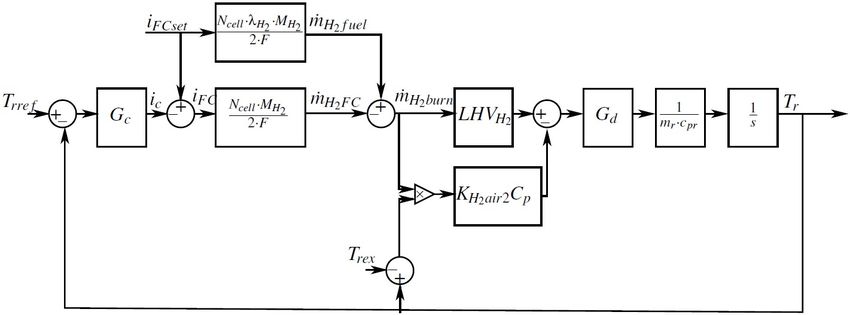
2
of the fuel tank. A smaller range extender will still contribute
significantly to the range of the vehicle as seen in Figure 1.
Here the effect of a 5 [kW ] range extender is plotted together
with the standard range. An assumed 15 minute warm-up
period, together with a soft start of the power output of the
range extender has been added to the simulation.
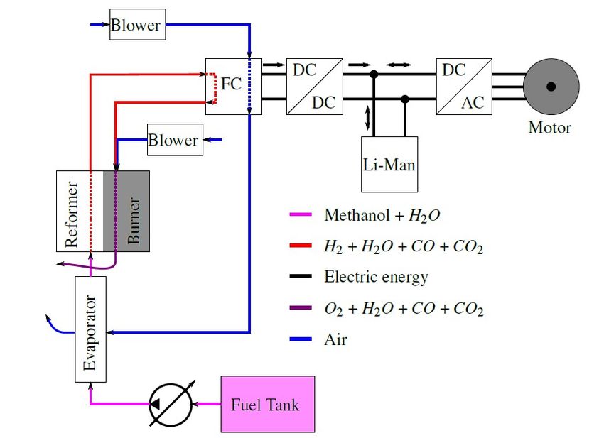
Figure 2. Conceptual drawing of the methanol fuel reformer, the fuel cell
system and the car’s existing electrical system.
The fuel pump is a membrane pump, which means that the
fuel flow in the system, Q f uel , is controlled by changing the
pump frequency. The fuel is pumped into an evaporator which
Figure 1. Battery capacity in [kW h] during maximum drive range with and uses the exhaust heat from the fuel cell to heat and vaporize the
without a 5000[W ] range extender.
fuel. In the reformer the fuel is superheated and reformed into
mainly hydrogen and carbon dioxide. The reactions which take
place in the reformer are pressure and temperature dependent.
A 5 [kW ] range extender is considered because a fuel cell The three reactions are: The Steam reformation process, the
system of this size is under development by Serenergy R . To decomposition process and the water gas shift or WGS [4][7,
give a forecast of the amount of fuel necessary a fuel cell p. 51]. The steam reformation process is:
system efficiency of 0.3 is assumed. A run time of 5.68 [h]
(neglecting warm-up time), a heating value for methanol of CH3 OH + H2 O CO2 + 3H2 (3)
4373 [W h/l] and a fuel mixture of 60% methanol and 40%
water, the fuel requirement for this range extender is: This is an endothermic process which requires heat. The
methanol decomposition process is:
5000[W ] · 5.68[h] CH3 OH CO + 2H2 (4)
Fuel = = 36[l] (2)
4373[W h/l] · 0.3 · 0.6 This is also an endothermic process which produces hydrogen
but also unwanted carbon monoxide. Equation 5 shows the
A fuel tank of 36 [l] is an acceptable size for the eCarver, WGS reaction.
hence the initial calculations indicate that a reformer based CO + H2 O CO2 + H2 (5)
fuel cell system is applicable as a range extender solution.
The WGS process is exothermic, meaning that it releases
heat. It converts some of the unwanted carbon monoxide. The
steam reformation and WGS processes require water to be
present, hence the water in the fuel. The fuel mixture of 60%vol
B. Fuel cell system methanol and 40%vol water can be expressed as a ratio on
mole basis. This is called the steam to carbon ratio (SC) and
The system which is treated in this paper is the H3-350 is 1:1.5 for the fuel used in this system. This indicates that
system produced by Serenergy R . It is a 350 [W ] system but there is a surplus of water for the chemical reaction, which
the technology is scalable and as mentioned above, a 5 [kW ] is favorable for the forward reaction of Equation 5 [4]. The
system is under development. overall process is endothermic, which means that a continuous
The methanol fuel system consists of a fuel pump, an evapo- energy supply to the reformer is required. This is achieved
rator and a reformer combined with a burner. The output gases by burning hydrogen catalytically. The fuel for the burner is
from the reformer are fed into the fuel cell. The electric output hydrogen from the reformation process that has passed through
from the fuel cell is connected to the DC-link of the vehicle the fuel cell unused. A normal approach to ensure a sufficient
through a controllable DC-DC converter. The main layout of fuel supply to the burner is to run the system with a fixed
the proposed system can be seen in Figure 2, together with hydrogen stoichiometry, λH2 , meaning that the hydrogen flow
the battery and motor controller of the electric vehicle. The increases linearly to both the fuel cell and the burner when
battery allows the power output of the fuel cell system to be the current draw is increased. By running the burner with
different than the instantaneous power demand of the vehicle. a surplus of hydrogen, the temperature can be controlled by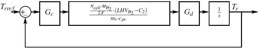
3

increasing the burner airflow to cool it down. This results in                 Where QH2 ,b is the energy flow from from the catalytic burning
an undesirable waste of fuel.                                                  of hydrogen in the burner:
To improve the efficiency of the system it is suggested to
regulate the reformer temperature by adjusting the current
drawn from the fuel cell. By increasing the current from the                                     QH2 ,b = ṁH2 ,b · LHVH2 · Gd (s)               (12)
fuel cell, without increasing the fuel flow, less hydrogen will
reach the burner and the temperature will decrease without                       Q f h,r is the power needed to superheat the fuel flow:
raising the airflow.
                                                                                                   Q f h,r = C p,mg · (Tr − Tex,e )              (13)
                                III. M ODELS
   Two types of models are developed in this paper, a dynamic                    Qair,r is the energy flow out of the reformer due to the
model and a linearized model. The dynamic model is used                        process air of the burner:
to simulate the performance of the system and the linearized
model is used for controller design.                                                       Qair,r = ṁair,r · c p,air · (Ta − Tex,r ) · Gd (s)   (14)

A. Dynamic model                                                                  Where the exhaust temperature of the burner Tex,r is mod-
                                                                               eled as a function of the reformer temperature:
  A dynamic model is derived and implemented in MATLAB
R
   Simulink to assess the performance of the reformer and fuel
                                                                                                        Tex,r = Tr · aex + bex                   (15)
cell system.
The mass-flow from the fuel pump is modeled as:
                                                                                 The energy flow for the overall endothermic reformation
                            ṁ f p = v f p · ρml · f f p                 (6)   process is modeled using Equation 16. The process requires:
                                                                               ∆H = 49.4 kJ/molCH3 OH to take place [4, p.90].
 The evaporator, which is basically a heat exchanger, is
modeled as the energy balance of a point mass [8]:
                                                                                                    ∆H
            1
                      Z                                                                   Qdc =            · (ṁCH3 OH − ṁCH3 OH,slip )         (16)
    Te =                  (Qair,e + Pe,e − Q f h,e − Qcond,e + Qcond,r,e )                         MCH3 OH
         me · c p,e
                                                                         (7)   where ṁCH3 OH,slip is the methanol which goes unreformed
   Where Qair,e is the heat supplied to the evaporator from                    through the reformer. The energy flow into the burner, has a
the air flow of the fuel cell cathode, modeled by Equation                     delay before it is transferred to the reformer. From empirical
8, under the assumption that the flow reaches the evaporator                   data, a transport delay and a first order filter are used to
temperature.                                                                   emulate the delay of this energy flow, shown in Equation 17.

                                                                                                                                1
                                                                                                   Gd (s) = e−s·tdelay ·                         (17)
                  Qair,e = ṁair,FC · c p,air · (TFC − Te )              (8)                                               τr · s + 1
   Q f h,e is the power required to heat, vaporize and superheat                  The electrical fuel cell model is based on the model pro-
the fuel from ambient to evaporator temperature.                               posed in [9] and [5] with the modifications proposed in [10].
                                                                               This model emulates the temperature of the fuel cell and the
                 Q f h,e =ṁ f p · [c p,ml · (T f e − Ta )                     output voltage as a function of the output current and the
                                                                               CO and H2 content of the gas. Therefore an estimator for
                             + c p,mg · (Tex,e − T f e ) + Lm ]          (9)
                                                                               the contents of the reformate gas is needed.
  Qcond,r,e is the conduction heat transferred in the piping                   ANFIS modeling is selected to estimate the gas content
between the reformer and the evaporator given by Equation                      because it can be trained on experimental data and emulate
10.                                                                            nonlinear relations. The ANFIS is trained using test data at
                                                                               different reformer temperatures and fuel flows covering the
                                                                               normal operating range. Four ANFIS predictors which use
                      Qcond,r,e = Ccond,r,e · (Tr − Te )                (10)   the temperature of the reformer and the fuel flow as inputs
   Heat loss to the surroundings (Qcond,e ) is modeled in the                  are trained. The outputs of the four ANFIS predictors for the
same manner as Qcond,r,e , i.e. radiation is neglected. The exit               reformed gas are:
temperature of the fuel from the evaporator is determined on                     •   xCO the carbon monoxide fraction.
the basis of experimental data to be: Tex,e = Te − 14, under                     •   ṁCH3 OH,s the methanol slip.
normal working conditions.                                                       •   ṁH2 the hydrogen mass flow.
   The thermal model of the reformer and burner is also                          •   ṁCO2 the carbon dioxide mass flow.
modeled as an energy balance of a point mass:
                                                                               A plot of the training data and the resulting output of the
            1
                      Z
    Tr =                  (QH2 ,b + Pe,r − Q f h,r − Qair,r − Qdc )     (11)   ANFIS predictor for the carbon monoxide concentration are
         mr · c p,r                                                            shown in Figure 3.
4
Input The simulation of the experiment results in an MSE of 3.19
Fuel, Temperature 400
300
Fuel ⋅ 1e6 [kg/s]
Tr [°C]
[◦C] which corresponds to 2.88%.
200 Figure 5 shows the simulated and measured reformer tem-
100 perature during a number of steps in the fuel flow.
0
0 2000 4000 6000 8000 10000 12000 14000 16000 18000
x 10
4 Output
2.5 450 vdotfp [ml/h]
ANFIS Output
2 Training Data Tr−sim [°C]
400
CO [ppm]
Temperature, Power, Pump flow
Tr−meas [°C]
1.5
350 Pe,r−meas [W]
1 QH [W]
,b−meas
300 2
0.5 Qair,b−meas [l/min]
0 250
0 2000 4000 6000 8000 10000 12000 14000 16000 18000
Time [s] 200
150
Figure 3. The output of this ANFIS model is the CO content of the reformate 100
gas in ppm and the inputs are the reformer temperature and the fuel flow. 50 MSET_r = 8.46° C
0
4000 4500 5000 5500 6000 6500 7000 7500
The four ANFIS predictors are evaluated using Mean Time [s]
Squared Error (MSE) on the data points in the training data,
the MSE in percent is with respect to the mean value of the Figure 5. Simulated and measured reformer temperature from the same
experiment as figure 4.
training data. The results are shown in Table I together with
the number of fuzzy membership functions employed in each
model. The simulation of the experiment results in an MSE of 8.02
[◦C] which corresponds to 2.70%.
Modeled parameter No. MF MSE MSE [%]
ṁH2 [kg/s] 3 8.1864e-008 1.6
Figure 6 shows the simulated and measured reformer ex-
ṁCO2 [kg/s] 3 5.9467e-007 1.56 haust temperature during a step in the reformer temperature.
ṁCH3 OH,s [kg/s] 4 5.0341e-007 17.7
xCO [ppm] 5 1.3049e+003 24.17
Table I 300
M EAN SQUARED ERROR OF THE FOUR ANFIS SYSTEMS .
250
Temperature [°C]
200
B. Validation of dynamic model 150
To optimize the parameters in the thermal-model, the ex- 100
perimental data is used as input to the model and the resulting Tex,r−sim [°C]
MSET = 3.34° C
50 Tr−meas [°C]
evaporator and reformer temperatures are observed. The model ex,r
Tex,r−meas [°C]
is then optimized to output temperatures similar to those ob- 0
1000 2000 3000 4000 5000 6000
Time [s]
served in the experiments. It is desired to achieve a simulated
evaporator and reformer temperature which is within an MSE
Figure 6. Measured reformer and exhaust temperature of the same test as
of 5% of the measured temperature in [◦C]. The model is used Figure 4, with estimated exhaust temperature using Equation 15, at different
without any controllers to stabilize the output, hence a small air flows, see the blue data in Figure 5.
deviation in the energy calculations can integrate over time to
become a larger steady state error. Therefore the measured test-
The MSE for the exhaust temperature in Figure 6 is 3.34
data that runs over several hours is used in smaller fractions
[◦C] corresponding to an error of 1.93% of the mean of the
for the validation. Figure 4 shows the simulated and measured
measured exhaust temperature. For all the performed tests the
evaporator temperature during a series of steps in the fuel flow.
MSE is within the 5% limit.
450 vdotfp [ml/h]
Te−sim [°C]
400
Te−meas [°C] IV. L INEAR MODEL
Temperature, Power, Flow
350 Pe,e−meas [W]
Qair,e−meas [W]
300
To design and implement the proposed Current Correction
250
Temperature Controller, a linear model of the thermal reformer
200
150
system is produced. The input to the linear model is the mass
100
flow of hydrogen and the output is the reformer temperature. A
MSET = 2.53° C
50
e
block diagram of a simplified thermal model and the proposed
0
1000 2000 3000 4000 5000 6000
temperature control scheme is shown in Figure 7. The model
Time [s]
is linearized around an operating point assuming a constant
Figure 4. Simulated and measured evaporator temperature from an exper-
ambient and evaporator temperature. The linear model will
iment where the fuel flow is stepped, and the evaporator is supplied by a only model the dynamics of the system accurately and not the
constant energy flow, in the form of hot air from an air flow controller. steady state values.5
that the reformer is not subjected to excessive temperatures
because these could be harmful. It is also important that the
steady state error is minimized to ensure that the reformation
process takes place at the desired temperature. The rise time
when subjected to a step input is used as an indicator for
the speed of the control system. The demands for the control
system are specified in Table II.
Parameter Demand Unit
Figure 7. Representation of the simplified thermal model of the reformer.
Max overshoot 1.5 [◦C]
Upper convergence limit 1.5 [◦C]
The needed hydrogen flow from the reformer, ṁH2 f uel , is Lower convergence limit 1.5 [◦C]
estimated using Equation 18 which calculates the hydrogen Rise time 100 [s]
Max controller output 30 %
flow consumed by the fuel cell, multiplied by the stoichio-
metric factor λH2 . Table II
D EMANDS FOR THE CONTROL SYSTEM .
ncell · MH2 · λH2 mol
ṁH2 f uel = · IFC (18)
2·F s
To avoid hydrogen combustion in the pipes leading to the The plant has a free integrator which comes from the
burner, a phenomena known as flashback, a minimum rela- summation of energy in the thermal mass of the reformer.
tionship between the burner air and burner hydrogen mass This implies that there will be no steady state error for step
flow must be fulfilled [10, p. 87]. Equation 19 shows this inputs if a P controller is used. This is not the case for
relationship. the real system because of the constant contribution which
was neglected when the linear model was constructed. It
ṁair,r,min
KH2 air2 = (19) is therefore necessary to use a PI controller to eliminate
ṁH2 ,b
steady state error. Table III shows some of the performance
It has been determined experimentally that a relationship of parameters of the linear system with the chosen controller.
115 is a safe minimum. This relationship has to be achieved
by predicting the hydrogen flow and setting the air flow Phase Margin 59 [deg]
appropriately. This prediction is made using the developed Gain Margin 16.7 [dB]
Rise time 46.4 [s]
ANFIS model. Gd contains the dynamics and the delay of Overshoot 15 [%]
the energy transfer between the burner and the reformer.
Table III
Linearizing the model around a constant current set-point P ERFORMANCE OF THE DESIGNED CONTROLLER IN THE LINEAR MODEL .
IFCset and reformer temperature, obtaining a single constant for
the burner hydrogen and air flow, yields the model in Figure
8.
An often used stability criterion is that the gain margin
should be at least 8 [dB] and the phase margin at least 50◦ [11,
p.323]. These demands are fulfilled and the control system is
considered to be stable.
Step Response
Figure 8. Block diagram of the linearized model and temperature controller 1.2 Upper Convergence limit
for the reformer temperature.
1
Lower Convergence limit
The linearization constant C2 is seen in Equation 20, where 0.8
Amplitude
Tr_lin is the linearization temperature of the reformer, and 0.6
Tex,r_lin is that of the reformer exhaust air. 0.4
C2 = KH2 air2 · c p,air · (Tr_lin − Tex,r_lin ) (20) 0.2
PI−controller
This linearized model is used to develop a controller. 0
0 100 200 300 400 500 600 700 800 900 1000
The performance of the controller will be verified using the Time (seconds)
dynamic model. This also serves as a verification of the linear
Figure 9. Closed loop step response of the linear model using the designed
model. controller.
V. C ONTROLLER
The controller output in the dynamic model is saturated at
A. Temperature controller ±5[A] which is ≈ 30% of the rated current. To avoid integrator
When choosing a controller it is important to determine the windup, the conditioning anti-windup scheme presented in
performance demands of the control system. It is important [12] is implemented.6
305
Step response of PI controller with anti windup is not acceptable since it can be harmful to the fuel cell, as
Trref
Temperature [°C]
300
Tr anode or cathode carbon corrosion can occur [7]. Therefore a
minimum stoichiometry of 1.2 is desired to avoid degradation.
295
To ensure this a dynamic saturation of the correction current
290
is implemented, using hydrogen mass flow prediction. The
285
6000 6100 6200 6300 6400 6500 6600
implemented dynamic saturation appears from Equation 21.
Time [s]
10
Ic ṁH2 est · 2 · F
Icsat =− − IFCset (21)
λH2 _lim · ncell · MH2
Current [A]
5
0
The estimated hydrogen flow ṁH2 est is calculated using the
developed ANFIS model.
−5
6000 6100 6200 6300 6400 6500 6600
Time [s]
Stoichiometry and correction current during temperature steps
Temperature [°C]
310
Trref
300 Tr
Figure 10. Simulated reformer temperature step response and correction
current output from the controller. 290
280
5800 6000 6200 6400 6600 6800 7000 7200 7400 7600 7800
Time [s]
Comparing the step responses plotted in Figure 9 and 10 of
Stoichiometry [−]
both the linear and dynamic model shows very similar results. 1.4 Stoichiometry
A 10 [◦C] step response applied to the dynamic model gives 1.2
an overshoot of 1.45 [◦C] which is an overshoot of 14.5%, 1
5800 6000 6200 6400 6600 6800 7000 7200 7400 7600 7800
and the rise time is 46.1 [s], which corresponds to the values Time [s]
in Table III. Hence the linear model is deemed valid and the Current [A] 2
Icset
0
system stable. Ic
−2
−4
5800 6000 6200 6400 6600 6800 7000 7200 7400 7600 7800
B. Fuel flow controller Time [s]
If the current correction scheme outlined above is used on
its own, it will lead to a steady state error between the current Figure 12. Negative temperature step response in the dynamic model with
set point and the fuel cell current. An outer control loop which static correction current saturation of ±5 [A]. Note that the stoichiometry falls
changes the fuel flow to make the correction current Ic zero below 1, which leads the fuel cell into anode starvation.
over a certain period of time is therefore implemented. This
controller will change the fuel flow to that required to maintain In Figure 13 the dynamic model is subjected to the same
the desired fuel cell current and reformer temperature. Figure step as in Figure 12, the temperature rise time is slower
11 shows the structure of this controller implemented in the because of the dynamic saturation limit, but the stoichiometry
system from Figure 7. is kept above 1.2 as intended. The fuel flow controller slowly
adjusts the pump frequency until the desired output current is
achieved with the smallest possible fuel flow for the system.
This is the case when the correction current is equal to zero.
Stoichiometry and correction current during temperature steps
Temperature [°C]
310
Trref
300 Tr
290
280
5800 6000 6200 6400 6600 6800 7000 7200 7400 7600 7800
Time [s]
Figure 11. Block diagram for the fuel flow controller Gc2 .
Stoichiometry [−]
1.4 Stoichiometry
1.2
A fuel flow controller only consisting of an integral part is
1
chosen, as a PI controller reacts immediately to an error, which
5800 6000 6200 6400 6600 6800 7000 7200 7400 7600 7800
is not the intention. The pump flow controller is supposed to Time [s]
adjust the pump flow slowly enough to allow for the reformer
Current [A]
1 Icset
Icsat
temperature controller to correct the change in temperature 0
Ic
caused by the change in fuel flow. −1
In Figure 12 a negative temperature step is performed. During −2
5800 6000 6200 6400 6600 6800 7000 7200 7400 7600 7800
Time [s]
a negative step the fuel cell current is increased to decrease
the hydrogen flow to the burner, this can cause starvation of
the fuel cell if the negative correction current is too large. As Figure 13. Negative temperature step response in the dynamic model with
is evident from the stoichiometry plot of Figure 12. Starvation dynamic correction current saturation, from Equation 21.7
VI. E FFICIENCY COMPARISON carbon monoxide tolerance, which improves the efficiency
To ensure that the system is operated at the optimal condi- further. It is concluded that the efficiency using Current Cor-
tions and to analyze the advantages of using the Current Cor- rection Temperature Control is 0.321 at the selected operating
rection Temperature Control method proposed in this paper, temperatures.
the efficiency of the system is analyzed. The system efficiency
is defined as the electric output power of the fuel cell divided B. Comparison to conventional blower control
by the Higher Heating Value (HHV) of the fuel. To assess how much efficiency is gained using Current
Correction Temperature Control, a more conventional reformer
A. Operating temperature temperature controller is developed which superimposes a
The methanol slip depends on the reformer temperature. cooling flow on the burner air flow. Table V shows the system
Higher temperatures means a lower slip but also higher losses efficiency using this controller.
due to convection. Higher reformation temperature also leads
Tr Efficiency TFC = 170 [◦C] Efficiency TFC = 180 [◦C]
to a larger carbon monoxide fraction in the reformate gas, 300 0.2270 0.2813
which lowers the fuel cell efficiency. The dynamic model is 290 0.2320 0.2834
therefore used to evaluate the system efficiency at different 280 0.2350 0.2848
270 0.2380 0.2853
operating temperatures. Two different fuel cell temperatures 260 0.2390 0.2841
are also investigated. Table IV shows the results of the 250 0.2400 0.2832
simulation. Table V
S YSTEM EFFICIENCY AT DIFFERENT REFORMER AND FUEL CELL
Tr Efficiency TFC = 170 [◦C] Efficiency TFC = 180 [◦C] TEMPERATURES USING BLOWER TEMPERATURE CONTROL .
300 0.2672 0.3190
290 0.2722 0.3210
280 0.2716 0.3192
270 0.2708 0.3161 The system efficiency using this controller is better at low
260 0.2671 0.3124
250 0.2661 0.3102
temperatures because it uses an over stoichiometry which
means that the higher methanol slip has no consequence in
Table IV
S YSTEM EFFICIENCY AT DIFFERENT REFORMER AND FUEL CELL
this model. For this comparison it is assumed that it does not
TEMPERATURES USING C URRENT C ORRECTION T EMPERATURE C ONTROL . hurt the fuel cell to have this methanol slip and the system
efficiency using blower control is set to 0.2858.
It is concluded that using current correction control raises the
The efficiency is highest at Tr = 290 [◦C]. To illustrate why system efficiency with a fuel cell temperature of 180 [◦C] from
this is the case, the reformate gas flow and the power lost due 0.2858 to 0.3210. This is an improvement of 3.52 percentage
to the anode voltage drop are plotted in Figure 14. points, which corresponds to a relative increase in efficiency
of 12.32%.
Reformate gas composition at different temperatures
Temperature [°C]
300 Trref
Tr
C. Using exhaust heat for cabin heating
280
260
In a petrol or diesel powered vehicle, the waste heat from
240 the engine is used to heat the cabin. This means that none of
Mass flow [g/s] fraction [−]
0.5 0.6 0.7 0.8 0.9 1 1.1 1.2 1.3 1.4 1.5 1.6
Time [s] x 10
4
the power produced by the engine is used for cabin heating.
0.015
In an purely electric vehicle, the energy used for cabin heating
0.01 xCO
mdotH
has to come from the batteries, which hurts the range of the
0.005 2
mdotCH OH,s
3
vehicle. This problem can be eliminated by using the exhaust
0
0.5 0.6 0.7 0.8 0.9 1 1.1 1.2 1.3 1.4 1.5 1.6 heat from a methanol powered range extender. The exhaust
Time [s] x 10
4
temperature of the evaporator is 102 [◦C] and the flow is
2.18e-3 [g/s]. With an ambient temperature of 10 [◦C] it is
40
Power [W]
Power loss anode
30
20 assumed that the exhaust air is cooled to half the temperature
difference meaning a temperature drop of 46 [◦C]. The power
10
0
0.5 0.6 0.7 0.8 0.9 1 1.1 1.2 1.3 1.4 1.5 1.6
Time [s] x 10
4
which can be exhumed from the air is modeled to be 114.7
[W ]. This makes the combined system efficiency 0.3980.
Assuming direct scalability between the tested system and the
Figure 14. Gas composition and power loss due to anode voltage drop at
different temperatures. 5 [kW ] system, which is under development by Serenergy R ,
the heating power would be 1.6 [kW ].
The carbon monoxide content is relatively large at 300 [◦C]
leading to a higher anode voltage drop and therefore a larger VII. C ONCLUSION
power loss [10]. The methanol slip is relatively small at both In this work an alternative reformer temperature controller
300 and 290 [◦C] leading to the optimal reformer temperature using Current Correction Temperature Control has been pro-
being 290 [◦C]. Higher fuel cell temperature leads to a higher posed. The stability of the controller was proven using a linear8
Pe,e Power from electric heater in evaporator [W ]
model and the performance was verified using a dynamic Pe,r Power from electric heater in reformer [W ]
model. The dynamic model has been verified experimentally tdelay Time delay [s]
and includes ANFIS models of the gas composition trained Ta Ambient temperature [K]
on experimental data. The system efficiency was investigated Te Evaporator temperature [K]
using the dynamic model for both a conventional blower con- Tex,e Evaporator exhaust temperature [K]
Tex,r Reformer exhaust temperature [K]
troller and for the proposed Current Correction Temperature
TFC Fuel cell temperature [K]
Controller. The system efficiency was found to be improved Tf e Boiling temperature of fuel [K]
from 0.2858 to 0.3210 which constitutes an improvement of Tr Reformer temperature [K]
12.32%. If the exhaust heat is used for cabin heating, the Trre f Reformer reference temperature [K]
combined efficiency can be pushed to 0.3980. It still remains to vf p Displacement of the fuel pump [m3 ]
test the Current Correction Temperature Controller in practice. vdot_ f p Fuel flow from the fuel pump [mL/h]
xCO Fractionel CO content of reformate gas [.]
∆H Reformation process energy [kJ/mol ]
ACKNOWLEDGMENT λH2 Hydrogen stoichiometry setpoint [.]
λH2 _lim Lower stoichiometry limit [.]
The authors would like to thank Søren Juhl Andreasen, ρml Density of liquid fuel [kg/m3 ]
Hamid Reza Shaker and Simon Lennart Sahlin for guidance, τr Time constant of Gd [s]
and the companies Lynx and Serenergy R for technical support
during the project. R EFERENCES
[1] eCarver by Lynx, http://www.lynxcars.com/, 2011, Manufacturer of elec-
tric vehicles.
N OMENCLATURE [2] European Commission - Joint Research Center, Well-to-Wheels analysis of
future automotive fuels and powertrains in the European context, Report
Version2b, 2006.
aex Exhaust temp coefficient [.] [3] Zhongliang Zhan, Worawarit Kobsiriphat, James R. Wilson, Manoj Pillai,
bex Exhaust temp coefficient [◦C] Ilwon Kim & Scott A. Barnett, Syngas Production By Coelectrolysis
C p,air Specific heat capacity of air [kJ/kg·K ] of CO2/H2O: The Basis for a Renewable Energy Cycle,2009, Scientific
C p,e Specific heat capacity of evaporator [kJ/kg·K ] paper, Department of Materials Science and Engineering, Northwestern
C p,r Specific heat capacity of reformer [kJ/kg·K ] University, Illinois.
C p,ml Specific heat capacity of liquid fuel [kJ/kg·K ] [4] Gu-Gon Park, Dong Joo Seo, Seok-Hee Park, Young-Gi Yoon, Chang-
C p,mg Specific heat capacity of evaporated fuel [kJ/kg·K ] Soo Kima and Wang-Lai Yoo, Development of microchannel methanol
steam reformer,2004, Scientific paper, Chemical Engineering Journal 101
Ccond,e Conduction coeff. from evaporator [W/K ] (2004) 87–92.
Ccond,r Conduction coeff. from reformer [W/K ] [5] Anders Risum Korsgaard, Mads Pagh Nielsen, Mads Bang & Søren
Ccond,r,e Conduction coeff. from reformer to evaporator [W/K ] Knudsen Kær, Modeling of CO influence in PBI electrolyte PEM fuel
C2 Linearization constant [kJ/kg] cells, 2006, Scientific paper, Proceedings of FUELCELL 2006, Institute
F Faradays constant [C/mol ] of Energy Technology, Aalborg University, DK-9220 Aalborg, Denmark
ffp Fuel pump frequency [Hz] [6] Serenergy R , http://www.serenergy.dk/, 2011, Manufacturer of HTPEM
Gd (s) Tf for energyflow from burner to reformer [.] fuel cell stacks and fuel cell power modules.
Gc Tf for temperature controller [A/K ] [7] Søren Juhl Andreasen, Design and Control of High Temperature PEM
Ic Correction current [A] Fuel Cell System, 2009, Ph.D dissertation from Aalborg University,
Institute of Energy Technology.
Icsat Lower correction current limit [A] [8] Yunus A. Cengel & Michael A. Boles, Thermodynamics, An Enginering
IFC Fuel cell current [A] Approach, 2007.
IFCset Fuel cell current set point [A] [9] Anders Risum Korsgaard, Rasmus Refshauge, Mads Pagh Nielsen, Mads
KH2 air2 Burner hydrogen to air mass flow ratio [.] Bang & Søren Knudsen Kær, Experimental characterization and mod-
LHVH2 Lower heating value of hydrogen [kJ/kg] eling of commercial polybenzimidazole-based MEA performance, 2006,
Lm Latent heat of fuel [kJ/kg] Scientific paper, Journal of Power Sources 162 (2006) 239–245, Institute
me Thermal mass of the evaporator [kg] of Energy Technology, Aalborg University, DK-9220 Aalborg, Denmark
mr Thermal mass of the reformer [kg] [10] Simon Lennart Sahlin & Jesper Kjær Sørensen, Control of methanol
MCH3 OH Molar mass of methanol [kg/mol ] fuelled HTPEM fuel cell system, 2009, 10th semester report from Aalborg
University, Institute of Energy Technology.
MH2 Molar mass of hydrogen [kg/mol ] [11] Charles L. Phillips & Royce D. Harbor, Feedback Control Systems, 4th
ṁair,FC Mass flow of air from fuel cell to evaporator [kg/s] edition, 2000.
ṁCH3 OH,s Mass flow of methanol slip [kg/s] [12] R. Hanus, M.Kinnaer & J.L. Henrotte, Conditioning Technique, a
ṁCO2 Mass flow of carbondioxide [kg/s] General Anti-windup and Bumpless Transfer Method, 1987, Scientific
ṁ f p Mass flow of fuel from pump [kg/s] paper, IFAC Automatica, Vol. 23, No. 6, pp. 729-739.
ṁH2 Mass flow of hydrogen in fuel [kg/s]
ṁH2 ,b Mass flow of hydrogen to burner [kg/s]
ṁH2 est Estimated mass flow of hydrogen to fuel cell [kg/s]
ncell Number for cells in fuel cell [.]
Qair,e Power in fuel cell airflow to evaporator [kJ/s]
Qair,r Power in fuel cell airflow to reformer [kJ/s]
Q f ,r Power in blower airflow to burner [kJ/s]
QH2 ,b Power to heat fuel flow in reformer [kJ/s]
Qdc Power to decompose fuel flow [kJ/s]
Q f ,h Power to heat and vaporize fuel flow in evap. [kJ/s]
Qcond,e Power loss by conduction from evaporator [kJ/s]
Qcond,r Power loss by conduction from reformer [kJ/s]
Qcond,r,e Power from reformer to evaporator in pipes [kJ/s]You can also read