Ultrahigh Resolution Scatterometer Winds near Hawaii - MDPI
←
→
Page content transcription
If your browser does not render page correctly, please read the page content below
remote sensing
Article
Ultrahigh Resolution Scatterometer Winds
near Hawaii
Nolan Hutchings 1,† , Thomas Kilpatrick 2 and David G. Long 1,†, *
 1    Department of Electrical & Computer Engineering, Brigham Young University, 450 EB, Provo, UT 84602,
      USA; nolanhutchings63@gmail.com
 2    Scripps Institution of Oceanography, University of California San Diego, 9500 Gilman Dr MC 0206, La Jolla,
      CA 92093, USA; tkilpatrick@ucsd.edu
 *    Correspondence: long@byu.edu
 †    These authors contributed equally to this work.

 Received: 8 January 2020; Accepted: 5 February 2020; Published: 8 February 2020

 Abstract: Hawaii regional climate model (HRCM), QuikSCAT, and ASCAT wind estimates are
 compared in the lee of Hawaii’s Big Island with the goal of understanding ultrahigh resolution (UHR)
 scatterometer wind retrieval capabilities in this area, which includes a reverse-flow toward the island
 in the lee of the predominate flow. A comparison of scatterometer measured σ0 and model predicted
 σ0 suggests that scatterometers can detect the reverse flow in the lee of the island; however, neither
 QuikSCAT- nor ASCAT-estimated winds consistently report this flow. Furthermore, the scatterometer
 UHR winds do not resolve the wind direction features predicted by the HRCM. Differences between
 scatterometer measured σ0 and HRCM predicted σ0 indicate possible error in the placement of key
 reverse flow features predicted by the HRCM. We find that coarse initialization fields and a large
 size median filter windows used in ambiguity selection can impede the accuracy of the UHR wind
 direction retrieval in this area, suggesting the need for further development of improved near-coastal
 ambiguity selection algorithms.

 Keywords: scatterometer; ocean winds; wind retrieval

1. Introduction
     Satellite radar instruments called wind scatterometers illuminate the Earth’s surface with
microwaves and measure the normalized radar cross-section (σ0 ) of the surface [1]. While the σ0
measurements prove useful for many applications such as iceberg tracking, ice classification, vegetation
classification, and soil moisture estimation [1–4], the scatterometer’s primary function is to estimate
the near-surface vector wind from the ocean σ0 measurements.
     From σ0 measured over the ocean, estimates of wind speed and direction can be made over the
open ocean by combining σ0 measurements taken from different azimuth angles [1]. Unlike wind
measurements from buoys, ships, and planes, scatterometers provide regular global wind vector
estimates over large regions of open ocean. The large coverage and availability of scatterometer data
proves useful for weather studies and prediction [1,5,6]. Traditional wind estimates are retrieved on
a coarse 12.5 km or 25 km grid (referred to as L2B estimates) and are excellent for understanding
large scale wind flow and other features. Wind estimates close to shore are discarded due to land
contamination of ocean σ0 [7].
     Ocean σ0 are related to wind speed and direction through a geophysical model function
(GMF) [1,8,9]. In the GMF, a single σ0 value corresponds to multiple wind speed and direction pairs.
Hence, multiple σ0 observed at different look angles are needed to narrow the solution space [10].
Even with multiple σ0 , this process results in two to four ambiguous wind vector solutions for each

Remote Sens. 2020, 12, 564; doi:10.3390/rs12030564                         www.mdpi.com/journal/remotesensing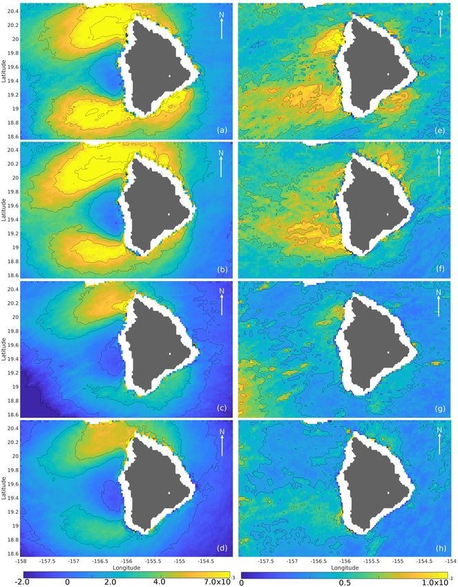
Remote Sens. 2020, 12, 564                                                                          2 of 15

resolution element (wind vector cell, WVC) [8]. From the ambiguous wind vector solutions, a final
wind field is chosen. This process of “ambiguity selection” begins by looking to an outside data
set, typically coarser in resolution, to initialize the ambiguity choices [10]. The initialization field,
sometimes referred to as a “nudging field”, ensures that general wind trends are present.
      After nudging, the wind ambiguities are further processed using a median filter based ambiguity
selection scheme [8,11,12]. The median filter based ambiguity selection scheme is not a true median
filter because it uses only the values available in the ambiguities. The median filter selection preserves
wind fronts and reduces noise, but as shown later, is limited by the size of the median filter window.
      With their high topography, the Hawaiian Islands greatly affect nearby wind conditions.
Orographic wind forcing near Hawaii not only influences local conditions, but extends far across the
Pacific Ocean [13,14]. Accurately observing and modeling these orographic winds is important in
understanding wind forcing of ocean circulation. Furthermore, improvements in Ultrahigh resolution
(UHR) wind retrieval can benefit other near-coastal areas with orographic wind forcing conditions.
      Wind estimation near the Hawaiian islands is a challenge for L2B coarse resolution estimates.
Complex fine resolution wind direction features and low wind speeds lead to systematic errors in L2B
wind estimation in the lee of Hawaii’s Big Island for both QuikSCAT and ASCAT [15]. Wind directions
in the lee of the Big Island can run counter to the prevailing trade winds, exhibiting a reverse flow
toward the island. The reverse flow has been both observed [16–18] and modeled [19,20]. The reverse
flow can be seen in the University of Hawaii’s numerical model winds [21]. The model is referred to as
the Hawaii regional climate model (HRCM), which provides predicted vector winds hourly on a 3 km
grid near the Hawaiian islands [19–22]. The reverse flow is only rarely observed in L2B winds [15].
      Figure 1 illustrates an HRCM wind field from a summer day and shows key wind features
expected in this area. Figure 1 shows trade winds blowing around the two peaks of the Big Island
creating regions of high wind speed to the north and south of the island and a low wind speed tail in
the lee (west side) of the island. The low wind speed tail is where the reverse flow is found. Due to the
consistency of the trade winds over Hawaii, generally, as in Figure 1, the reverse flow is found on the
west side of the island. However, the reverse flow phenomenon can be observed on other sides of the
island, depending on prevailing wind. The angle and length of the reverse flow region depends on
the direction and speed of the prevailing wind flow. The reverse flow region can extend as far out as
50–100 km from the shore [15,16].

      Figure 1. An example HRCM 3 km hourly wind vector field from 3:00 a.m. 26 June 2003. Wind speed
      is shown in color and wind direction quivers are downsampled and unit length. The land mask is
      shown in white. The reverse flow can be seen on the west side of the Big Island.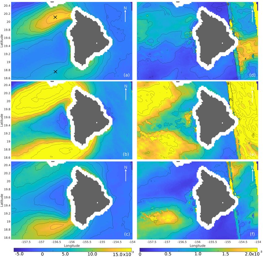
Remote Sens. 2020, 12, 564                                                                          3 of 15

     In the case of Figure 1, the model shows a reverse flow resulting from the formation of one
vortex. Often, multiple vortices (counter clockwise and/or clockwise) contribute to the reverse flow.
The locations and intensities of the vortices vary with changing wind flow.
     Resolution enhancement and reconstruction techniques enable estimation of winds on an
ultrahigh resolution (UHR) 2.5 km or 1.25 km grid [23–25]. UHR products have been produced for
QuikSCAT [25–29], RapidSCAT [30], and ASCAT [31,32]. UHR wind processing reveals finer resolution
detail of ocean wind phenomena and gives valuable insight to close to shore wind phenomena. Finer
resolution wind products allow wind estimation closer to shore through land contamination removal
(LCR) [7,32].
     This paper explores the UHR capabilities of QuikSCAT at 2.5 km and ASCAT at 1.25 km to
resolve the complex wind features in the lee of the Hawaii’s Big Island. In Section 2, a comparison
between QuikSCAT and ASCAT UHR winds and HRCM winds is outlined. In Section 3, scatterometer
measured σ0 are compared to model predicted σ0 . Section 4 shows the effects of the nudging field and
median filter-based ambiguity selection scheme on UHR scatterometer wind fields. Conclusions are
discussed in Section 5.

2. Scatterometer UHR Wind Estimates in the Lee of the Big Island
      In this paper, QuikSCAT and ASCAT passes from January 1, 2007 to December 31, 2008 are
considered for comparison with HRCM winds. The region of interest is between 20.50◦ and 18.75◦
latitude and −154◦ and −158◦ longitude around the Big Island. The high variability of winds in the
lee of the Big Island necessitates a close temporal collocation. In this analysis, only QuikSCAT passes
within 10 minutes and ASCAT passes within 20 minutes of the HRCM wind fields are used. ASCAT
orbits have a broader collocation window because only a few orbits are within 10 minutes of the
HRCM winds. For consistency, only scatterometer orbits with mean trade wind flow of around 270◦
that puts the reverse flow on the west side of the island are considered. From those years, a total of 276
QuikSCAT and 236 ASCAT passes are studied.
      We do not expect a perfect correspondence between the QuikSCAT and ASCAT observations
and HRCM winds because the HRCM winds are constrained only by observations at the lateral
boundaries. Thus, spontaneous behavior in the lee vortices and reverse flow shown by the model
likely may not match the scatterometer observations. Nevertheless, the HRCM winds are a useful
tool for comparison. It is important to note that HRCM winds predict wind speeds well below 5 m/s,
a range where scatterometers are less accurate due to lower SNR [33]. Scatterometer winds below
2 m/s are considered unreliable.
      HRCM provides winds near and over the islands; however, scatterometer wind retrieval is limited
to the ocean sufficiently far from land. For this reason, comparisons with UHR winds consider only
HRCM winds outside of the scatterometer ocean near-coastal zone land contamination buffer. In the
following, QuikSCAT UHR wind speeds and directions are first compared with the HRCM winds.
Then, a comparison of ASCAT UHR wind vectors with HRCM winds concludes. While we do compare
the wind speeds, the focus of the analysis is wind directions.
      Figure 2a compares collocated QuikSCAT UHR and HRCM wind speeds (all collocations are
within 2.5 km). The wind speeds between the two compare well. We note that the global mean wind
speed over the open ocean is approximately 7 m/s. At low wind speeds, QuikSCAT wind speed
estimates are biased somewhat higher compared to the model predicted speeds. Figure 2b compares
QuikSCAT UHR wind directions with HRCM wind directions. From the figure, it is apparent that
the trade winds (around 270◦ ) dominate the UHR wind direction field even when HRCM suggests
directions other than the trade winds. QuikSCAT UHR winds do not show the reverse flow or vortex
features that are included in the HRCM winds.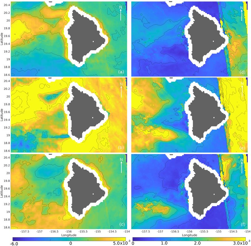
Remote Sens. 2020, 12, 564                                                                          4 of 15

      Figure 2. Density plots of QuikSCAT UHR wind speeds (a) and directions (b) plotted versus HRCM
      winds. A y = x line is included in each plot for reference.

     Figure 3 compares ASCAT UHR wind speeds and directions to HRCM winds (all collocations
are within 1.25 km). ASCAT UHR and HRCM wind speeds show a similar distribution to that
shown in Figure 2, though, for these particular ASCAT passes, the mean observed wind speed is
somewhat higher than the mean QuikSCAT winds. Figure 3 shows that ASCAT wind directions are
also dominated by trade wind flow and do not resolve the reverse flow and wind direction features of
the HRCM winds.

      Figure 3. ASCAT UHR wind speeds (a) and directions (b) collocated with HRCM winds. A y = x line
      is included in each plot for reference.
Remote Sens. 2020, 12, 564 5 of 15
In both cases, the scatterometer wind directions do not match well what the HRCM winds predict.
In particular, scatterometer winds do not show the reverse flow and vortices seen in the HRCM winds.
While the HRCM winds do show reverse flow and vortices, the true locations of any vortices and
reverse flow cannot be verified. With no truth data, it is difficult to draw too many conclusions from
the above analysis. These results do show, however, that the reverse flow and vortices are not resolved
in current UHR wind retrieval for QuikSCAT and ASCAT. In the next section, we turn to an analysis of
σ0 to further compare UHR products with the HRCM.
3. Comparison of Scatterometer Measured σ0 and Model Predicted σ0
Scatterometer measured σ0 are useful to examine because they are directly related to wind
stress [34]. The measurements are noisy, but they are unaffected by imperfect wind retrieval and
ambiguity selection routines. In this section, scatterometer measured σ0 are compared with predicted
σ0 from HRCM and European Centre for Medium-Range Weather Forecasts numerical weather
prediction (NWP) winds. The predicted σ0 values are generated for each model wind set using the the
QuikSCAT QMOD3 and ASCAT CMOD5 GMFs [8,9].
Comparison between the measured σ0 and HRCM predicted σ0 can show if the scatterometers’ σ0
measurements are possibly detecting the reverse flow and vortices. The coarse NWP wind fields show
only the trade wind flow and are a good baseline comparison to see if scatterometer measured σ0 are
detecting disturbances in the trade wind flow. The area of interest for this study is the same as in the
previous section. For consistency, only scatterometer passes with mean trade wind flow of around 270◦
that puts the reverse flow on the west side of the island are considered. The same temporal collocation
criteria are used in this comparison as in Section 2. However, additional stipulations are applied to the
scatterometer passes considered for this analysis.
QuikSCAT’s rotating pencil beam results in changing antenna observation angles across the swath.
Thus, only QuikSCAT passes with similar antenna look angles are considered. Similarly, ASCAT’s left
and right swaths have sufficiently different azimuth angles and are compared separately. Furthermore,
the incidence angle of fan beam scatterometers changes across the swath for each beam so passes
over Hawaii should be compared with like incidence angles. Only the left swath measurements and
passes with similar incidence angles over Hawaii are used in this study. This results in a total of 104
QuikSCAT orbits and 44 ASCAT orbits for analysis. First, QuikSCAT is compared to HRCM and NWP
predicted σ0 in Section 3.1; a comparison between ASCAT σ0 and predicted σ0 from the models follows
in Section 3.2.
3.1. QuikSCAT versus Model Predicted σ0
The average difference between the QuikSCAT measured σ0 and HRCM QMOD3 predicted σ0
for each “flavor” of σ0 is shown in Figure 4a–d. The four flavors of σ0 for pencil beam scatterometers
are vertical polarized fore looking (VF), vertical polarized aft looking (VA), horizontal polarized fore
looking (HF), and horizontal polarized aft looking (HA). The flavors are analyzed separately because
of the different effects azimuth angle and polarization have on σ0 . The first row in Figure 4 shows VF,
the second VA, the third HF, and the fourth row shows HA.Remote Sens. 2020, 12, 564 6 of 15
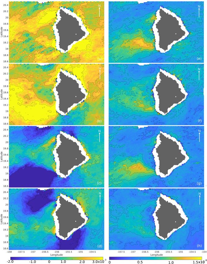
Figure 4. Panels (a–d) show the average difference in linear values between measured QuikSCAT σ0
and HRCM predicted σ0 for each flavor of σ0 ; (e–h) show the standard deviation of the difference
between measured QuikSCAT σ0 and HRCM predicted σ0 normalized by QuikSCAT average wind
speeds in linear values. The first row shows values for VF, the second is VA, the third HF, and the
fourth row is HA. Land is shown in gray and the land contamination buffer in white.
Despite the differences in the high wind speed regions, there is a low mean difference immediately
west of the Big Island seen in all polarizations. This is expected because, even if the two data sets have
different orientations for the low wind speed tail, the part immediately behind the island is commonRemote Sens. 2020, 12, 564 7 of 15
between them. However, the low difference is interesting because the QuikSCAT ambiguity-selected
winds in this area are generally 180◦ opposite of the HRCM directions. The σ0 agreeing in this area
suggests that QuikSCAT σ0 may be detecting the reverse flow, even if the selected QuikSCAT wind
directions do not match the model winds there. The differences in wind speed and direction between
the two may be because the wind ambiguity selection is in error in the scatterometer winds. It is
important to note that the wake of the island is a low speed region, so we do expect a lower difference
in this area due to lower σ0 values since σ0 is directly proportional to a power of the wind speed.
Figure 4e–h shows the standard deviation of the difference between the σ0 normalized by
QuikSCAT average wind speeds. We normalize with respect to QuikSCAT average wind speeds
because σ0 values are more variable as wind speed increases. This normalization has the effect of
lowering the standard deviation values in high wind speed areas. This partially removes the effect of
wind speed on the comparison.
In Figure 4e–h, the standard deviation is the highest in the southern high wind speed area.
Variation in the differences in the high wind speed area suggests that HRCM’s predicted wind tail
and reverse flow features do not match what QuikSCAT is detecting. The low standard deviation
directly west of the island indicates that both wind fields are consistently close in that area while
the low difference in σ0 and low standard deviation values suggest that QuikSCAT σ0 is detecting a
reverse flow.
The comparisons between the two data sets are clearly dependent on azimuth angle as seen by
the “mirroring” of the differences in the north and south high wind speed areas between the fore and
aft observations (compare Figure 4a and b or c and d). The effect of azimuth angle on σ0 is explained
below with some ASCAT measurements near the Big Island. We show this with ASCAT measurements
and NWP predicted σ0 because of how clearly they illustrate the effect of azimuth angle.
σ0 is a function of wind speed and χ (difference between antenna look angle and wind direction).
As wind speed increases so does the variability of σ0 with respect to χ. This can be seen in Figure 5a
in the CMOD5 σ0 curves plotted at different wind speeds. At 5 m/s, σ0 varies little as χ changes.
In contrast, at 15 m/s, the σ0 span a much larger range of values as χ changes.
In Figure 5a–c, ASCAT σ0 values at a point in the north (red) and in the south (blue) high wind
speed areas are plotted versus χ. The ASCAT selected wind speeds and directions of the north and
south locations are similar to each other, but the σ0 at those locations vary slightly due to χ.
Figure 5d–f show NWP predicted σ0 taken from the same north and south locations as the ASCAT
measurements. The NWP wind speeds and directions at the north and south locations are similar
to each other. In general, the reported NWP wind speeds are much lower than that of ASCAT and
fall on a σ0 curve that does not vary much with χ. Comparing a and d shows that there is a greater
difference between the ASCAT measured σ0 and NWP predicted σ0 at the north end. In contrast, the
σ0 at the southern end have a relatively small difference. A similar comparison of a different beam in c
and f shows that there is a greater difference between σ0 at the southern end and the difference at the
northern end is relatively small. In the mid antenna look (b and e), both north and south points have
similar differences in σ0 .
The change in differences in σ0 is explained by a change in antenna azimuth look angle which
affects χ. The ASCAT and NWP wind speeds and directions are different but how well that shows up
in the σ0 depends on the look angle. This effect can be seen to varying degrees in Figure 4 and other
figures in this section. The high variability of HRCM winds makes it difficult to precisely identify this
effect, but artifacts can still be seen.Remote Sens. 2020, 12, 564 8 of 15
Figure 5. ASCAT σ0 from multiple revs from a point (see Figure 8 a) in the north high wind speed
region and a point in the south high wind speed region are plotted for fore (a), mid (b), and aft (c) looks.
Corresponding NWP predicted σ0 are shown in (d–f) for the same beams. σ0 curves at 50◦ incidence
angle for CMOD5 for 5, 10, and 15 m/s are plotted in each panel for reference. Error bars showing the
average difference between ASCAT measured σ0 and NWP predicted σ0 and the standard deviation of
the differences are plotted in black.
Measured QuikSCAT σ0 are compared with coarse NWP predicted σ0 . Figure 6a–d shows the
average difference between measured QuikSCAT σ0 and QMOD3 NWP predicted σ0 . As expected,
the average differences show that NWP is not modeling what QuikSCAT is detecting. There are large
differences in the high wind speed regions, especially for the vertical polarization. Both polarizations
have a low average difference immediately west of the Big Island. The horizontal polarization shows
differences in the same areas but with smaller differences on average. This is consistent with the the
QuikSCAT horizontal polarization being lower than the HRCM σ0 seen in Figure 4c,d.
Figure 6e–h show the standard deviation of the differences for QuikSCAT and NWP σ0 normalized
by QuikSCAT average wind speeds. There are high standard deviation values (especially for vertical
polarization) west of the island even in the area immediately behind the island where a reverse flow is
expected. The disagreement between NWP predicted σ0 (which represent only the trade wind flow)
and QuikSCAT σ0 measurements further suggests that QuikSCAT σ0 are possibly detecting a reverse
flow and vortices.Remote Sens. 2020, 12, 564 9 of 15
Figure 6. Panels (a–d) show the average difference in linear values between measured QuikSCAT σ0
and NWP predicted σ0 for different flavors of σ0 ; (e–h) show the normalized standard deviation in
linear values between measured QuikSCAT σ0 and NWP predicted σ0 . The first row is VF, second is
VA, third HF, and the fourth row HA. The land is shown in gray and the land contamination buffer is
shown in white.Remote Sens. 2020, 12, 564 10 of 15
3.2. ASCAT versus Model Predicted σ0
The average difference between the ASCAT measured σ0 and HRCM CMOD5 predicted σ0 is
shown in Figure 7. The near vertical boundary feature directly right of the island is an artifact resulting
from the swath edge in different passes where there is limited coverage from ASCAT passes. Data
from that area right of the island can be ignored.
Figure 7. The average difference between linear values of measured ASCAT σ0 and HRCM predicted
σ0 shown for fore (a), mid (b), and aft (c) beams. Corresponding normalized standard deviation of
the difference values are shown to the right in panels (d–f). The land is shown in gray and the land
contamination buffer is shown in white.
Like the QuikSCAT comparison, larger differences in σ0 can be seen in the high wind speed areas.
The effects of azimuth angle can be seen especially when comparing the fore and aft azimuth looks.
Immediately west of the island, the average differences and standard deviation values are low for all
looks. This is interesting because, like QuikSCAT, ASCAT ambiguity-selected wind directions do not
show the reverse flow. The low average difference and low normalized standard deviation values west
of the island suggest that ASCAT can be detecting the reverse flow. Imperfect ambiguity selection may
be why ASCAT winds do not show this feature. The variance in differences in the high wind speed
areas suggest that the orientation of the wind speed tail and placement of vortices by HRCM does not
match what ASCAT σ0 is detecting.Remote Sens. 2020, 12, 564 11 of 15
ASCAT measured σ0 and NWP predicted σ0 are compared in Figure 8. ASCAT σ0 show high
differences from NWP σ0 in the high wind speed regions and low differences immediately west of the
island. The variation seen immediately west of the island suggests that ASCAT σ0 can be detecting
something other than the trade wind flow.
Figure 8. The average difference between linear values of measured ASCAT σ0 and NWP predicted
σ0 shown for fore (a), mid (b), and aft (c) beams. Corresponding normalized standard deviation of
the difference values are shown to the right in panels (d–f). The land is shown in gray and the land
contamination buffer is shown in white. The Xs in (a) indicate where the wind speeds are taken from
for the plots in Figure 5.
3.3. Summary
Low differences in σ0 and low standard deviation values compared to HRCM predicted σ0
immediately west of the island suggest that the scatterometer σ0 can be detecting the reverse flow.
Comparison with the coarse NWP winds supports the idea that UHR σ0 from both sensors are detecting
the island induced perturbation of trade wind flow. Higher difference in σ0 and standard deviation
values in the HRCM comparisons in the high wind speed areas suggest that HRCM is misplacing keyRemote Sens. 2020, 12, 564 12 of 15
wind features. The following section details why the ambiguity-selected scatterometer wind fields may
not show the reverse flow wind features despite these features possibly being present in the σ0 field.
4. Nudging Field and Median Filter Window Size
The nudging field and median filter-based ambiguity selection scheme have a significant effect on
the ambiguity-selected scatterometer wind field. They ensure general wind trends are present, but also
smooth the final result. In [15], Kilpatrick et al. identify the nudging field and median filter window
size as potential problems for wind retrieval in this area for coarse resolution estimates. In this section,
we explore the effects of nudge winds and median filter window size on UHR estimates.
We employ simulation to explore the effects of the nudging field and median filter window size
on UHR wind estimation in the lee of the Big Island. Simulated σ0 measurements are created from fine
resolution HRCM winds using the QMOD3 GMF. Monte Carlo noise is added to the σ0 measurements.
The noisy σ0 measurements are then processed using traditional QuikSCAT UHR processing.
At each UHR WVC, wind retrieval results in two to four ambiguous wind vector solutions.
Among the ambiguous solutions are the wind speed and direction values that are close to the true
wind model values. Those ambiguities are the desired result of ambiguity selection. We chose to focus
on QuikSCAT for this analysis; however, ASCAT yields similar results.
We first examine the effects of the nudging field. Traditional QuikSCAT UHR wind estimation
uses L2B wind fields as a nudging fields and L2B is nudged with NWP wind fields. Consequently,
UHR is indirectly nudged with coarse 50 km NWP model winds. Below, we contrast coarse and high
resolution nudging fields.
Figure 9 shows a simulated HRCM wind field nudged with an L2B wind field. Where we expect
the directions in (a) to show the reverse flow, there are no reverse flow features. Alternatively, choosing
the original high resolution HRCM wind field as a nudging field reveals the expected wind features.
Comparing (a) and (c) reveals that the ambiguities of the WVCs in lee of the Big Island can represent the
reverse flow feature, the difference being the nudging field. Thus, key features can be misrepresented
or absent in the ambiguity-selected wind field if the nudging field is low resolution.
After the ambiguous field is nudged, it is processed with the median filter-based ambiguity
selection scheme. As mentioned earlier, following the standard approach, a median filter is chosen
because it reduces noise and preserves wind fronts. Figure 9b is the L2B nudged field that has been
median filtered with a 42.5 km (17 x 17 UHR WVC) window. Figure 9d shows the HRCM nudged field
median filtered with the same window. The main wind direction features (i.e., trade wind flow and/or
reverse flow) in (a) and (c) are preserved in (b) and (d), respectively. The median filtered field in (a)
does not show the reverse flow because it was not there to begin with. The filter can only preserve and
refine what is already there. The reverse flow in (b) is preserved in (d) after the median filter.
The median filter window size affects how well features are resolved. If the median filter window
is large, small features relative to the window can be lost. A window size that is too small can be
dominated by noise and choose incorrect ambiguities. Figure 10 shows Figure 9 panels (c) and (d) but
in a gray scale wind direction field to better illustrate this point. Figure 10a shows the truth nudged
field before filtering. Note the reverse flow in the lee of the Big Island and wind features near the
other islands (boxed in red). Figure 10b shows the field after filtering with the same 42.5 km window.
The relatively large reverse flow from (a) is still present in (b), but the smaller features (circled) near
the other islands are filtered away. These results confirm that the median filter can preserve the reverse
flow feature only if the feature is in the nudging field to begin with and the window size is not too
large relative to the feature.Remote Sens. 2020, 12, 564 13 of 15
Figure 9. Simulated HRCM wind field nudged with an L2B field (a), simulated field nudged with
L2B and median filtered (b), simulated field nudged with the true field (c), simulated field nudged
with true field and median filtered (d). The median filter window size is 42.5 km (17 x 17 UHR WVC).
Downsampled wind direction quivers are shown in all panels.
Figure 10. QuikSCAT UHR-derived wind direction fields for different median filter window sizes.
(a) shows a swath oriented wind direction field of a simulated HRCM wind field nudged with the
true wind field. (b) shows (a) processed with a 42.5 km (17 x 17 UHR WVC) median filter window.
Note how the dark features that differ from the mean flow (circled within the red box) in (a) disappear
in (b) after filtering. The land mask is shown in white and the colorbar denotes the wind direction
in degrees.Remote Sens. 2020, 12, 564 14 of 15
5. Discussion and Conclusions
In the open ocean, QuikSCAT and ASCAT L2B and UHR processing have been proven to provide
accurate estimates of ocean wind vectors. The lee of Hawaii’s Big Island presents a challenging case for
scatterometer wind retrieval due to proximity to land and the fine scale of the expected wind features.
In previous work, L2B has been shown to not resolve the complex wind features in this area [15].
This paper shows that selected ambiguity QuikSCAT and ASCAT UHR winds also do not resolve
the reverse flow and vortices in the wind fields as predicted by HRCM. However, comparison of
scatterometer measured σ0 to HRCM predicted σ0 show that the scatterometer σ0 can be detecting the
reverse flow features. The σ0 analysis also suggests that HRCM winds are inaccurately predicting the
locations of key reverse flow features compared to the scatterometer σ0 . It is thought that incorporating
high resolution scatterometer data into the HRCM could result in better wind prediction.
The reverse flow features may be missing in the scatterometer ambiguity-selected wind field
due to the coarse resolution of the nudging fields and the large window size for the median filter in
the UHR ambiguity selection, which causes erroneous ambiguity selection leading to wind direction
errors. To improve UHR wind retrieval in this area, a better representation of fine scale features near
Hawaii is needed. This can be provided by improved HRCM winds used to nudge the scatterometer
ambiguity selection.
Author Contributions: Conceptualization and methodology, N.H. and D.G.L.; validation, T.K.; writing—original
draft preparation, N.H.; writing—review and editing, D.G.L. and T.K. All authors have read and agreed to the
published version of the manuscript.
Funding: This research was partially funded by NASA Grants No. 80NSSC19K0057 and NNX14AL83Gl.
Acknowledgments: UHR wind products can be provided on request through the Scatterometer Climate Record
Pathfinder (SCP) at www.scp.byu.edu.
Conflicts of Interest: The authors declare no conflict of interest.
References
1. Ulaby, F.T.; Long, D.G. Microwave Radar and Radiometric Remote Sensing; The University of Michigan Press:
Ann Arbor, MI, USA, 2014.
2. Long, D.G. Polar Applications of Spaceborne Scatterometers. IEEE J. Sel. Top. Appl. Earth Observ. 2017,
10, 2307–2320. [CrossRef] [PubMed]
3. Lindell, D.B.; Long, D.G. High-Resolution Soil Moisture Retrieval with ASCAT. IEEE Geosci. Remote Sens.
Lett. 2016, 13, 972–976. [CrossRef]
4. Lindell, D.; Long, D. Multiyear Arctic ice classification using ASCAT and SSMIS. Remote Sens. 2016, 8, 294.
[CrossRef]
5. Chang, P.S.; Jelenak, Z.; Sienkiewicz, J.M.; Knabb, R.; Brennan, M.J.; Long, D.G. Operational use and impact
of satellite remotely sensed ocean surface vector winds in the marine warning and forecasting environment.
Oceanography 2009, 22, 194–207. [CrossRef]
6. Wentz, F.J.; Ricciardulli, L.; Rodriguez, E.; Stiles, B.W.; Bourassa, M.A.; Long, D.G.; Hoffman, R.N.;
Stoffelen, A.; Verhoef, A.; O’Neill, L.W.; et al. Evaluating and extending the ocean wind climate data
record. IEEE J. Sel. Top. Appl. Earth Observ. 2017, 10, 2165–2185. [CrossRef] [PubMed]
7. Owen, M.P.; Long, D.G. Land Contamination Compensation for QuikSCAT Near-Coastal Wind Retrieval.
IEEE Trans. Geoscie. Remote Sens. 2009, 47, 839–850. [CrossRef]
8. Physical Oceanography Distributed Active Archive Center (PO.DAAC). Seawind’s User Guide; Rev. 3.0;
Physical Oceanography Distributed Active Archive Center: Pasadena, CA, USA, 2006.
9. Hersbach, H.; Stoffelen, A.; de Haan, S. An improved C-band scatterometer ocean geophysical model
function: CMOD5. J. Geophys. Res. Oceans 2007, 112. [CrossRef]
10. Naderi, F.M.; Freilich, M.H.; Long, D.G. Spaceborne radar measurement of wind velocity over the ocean-an
overview of the NSCAT scatterometer system. Proc. IEEE 1991, 79, 850–866. [CrossRef]
11. Shaffer, S.J.; Dunbar, R.S.; Hsiao, S.V.; Long, D.G. A median-filter-based ambiguity removal algorithm for
NSCAT. IEEE Trans. Geosci. Remote Sens. 1991, 29, 167–174. [CrossRef]Remote Sens. 2020, 12, 564 15 of 15
12. Schultz, H. A circular median filter approach for resolving directional ambiguities in wind fields retrieved
from spaceborne scatterometer data. J. Geophys. Res. 1990, 95, 5291–5303. [CrossRef]
13. Xie, S.P.; Liu, W.T.; Liu, Q.; Nonaka, M. Far-reaching effects of the Hawaiian islands on the Pacific
Ocean-atmosphere system. Science 2001, 292, 2057–2060. [CrossRef] [PubMed]
14. Sakamoto, T.T.; Sumi, A.; Emori, S.; Nishimura, T.; Hasumi, H.; Suzuki, T.; Kimoto, M. Far-reaching effects
of the Hawaiian Islands in the CCSR/NIES/FRCGC high-resolution climate model. Geophys. Res. Lett. 2004,
12. [CrossRef]
15. Kilpatrick, T.; Xie, S.; Tokinaga, H.; Long, D.; Hutchings, N. Systematic scatterometer wind errors near
coastal mountains. Earth Space Sci. 2019, 6, 1900–1924. [CrossRef] [PubMed]
16. Nickerson, E.C.; Dias, M.A. On the existence of atmospheric vortices downwind of Hawaii during the
HAMEC project. J. Appl. Meteorol. 1981, 20, 868–873. [CrossRef]
17. Smith, R.B.; Grubišić, V. Aerial observations of Hawaii’s wake. J. Atmos. Sci. 1993, 50, 3728–3750. [CrossRef]
18. Patzert, W.C. Eddies in Hawaiian Waters; Technical report; Hawaii Inst of Geophysics: Honolulu, HI, USA,
1969.
19. Zhang, C.; Yuqing Wang, A.L.; Hamilton, K. Configuration and evaluation of the WRF model for the study
of Hawaiian regional climate. Mon. Weather Rev. 2012, 140, 3259–3277. [CrossRef]
20. Yang, J.; Zhang, J. Evaluation of ISS-RapidScat wind vectors using buoys and ASCAT data. Remote Sens.
2018, 10, 648. [CrossRef]
21. Asia-Pacific Data Research Center. 2019. Available online: http://apdrc.soest.hawaii.edu/ (accessed on
30 January 2020).
22. Zhang, C.; Wang, Y.; Hamilton, K.; Lauer, A. Dynamical downscaling of the climate for the Hawaiian Islands.
Part I: Present day. J. Clim. 2016, 29, 3027–3048. [CrossRef]
23. Lindsley, R.; Long, D.G. Enhanced-Resolution Reconstruction of ASCAT Backscatter Measurements.
IEEE Trans. Geosci. Remote Sens. 2016, 54, 2589–2601. [CrossRef]
24. Williams, B.A.; Long, D.G. A reconstruction approach to scatterometer wind vector field retrieval. IEEE Trans.
Geosci. Remote Sens. 2011, 49, 1850–1864. [CrossRef]
25. Plagge, A.; Vandemark, D.C.; Long, D.G. Coastal validation of ultra-high resolution wind vector retrieval
from QuikSCAT in the Gulf of Maine. IEEE Geosci. Remote Sens. Lett. 2009, 6, 413–417. [CrossRef]
26. Williams, B.A.; Owen, M.P.; Long, D.G. The ultra high resolution QuikSCAT product. In Proceedings of the
2009 IEEE Radar Conference, Pasadena, CA, USA, 4–8 May 2009; pp. 1–6. [CrossRef]
27. Williams, B.A.; Long, D.G. Estimation of Hurricane Winds from SeaWinds at Ultra High Resolution.
IEEE Trans. Geosci. Remote Sens. 2008, 46, 2924–2935. [CrossRef]
28. Owen, M.P.; Long, D.G. Simultaneous Wind and Rain Estimation for QuikSCAT at Ultra-High Resolution.
IEEE Trans. Geosci. Remote Sens. 2011, 49, 1865–1878. [CrossRef]
29. Owen, M.P.; Long, D.G. Prior Selection for QuikSCAT Ultra-High Resolution Wind and Rain Retrieval.
IEEE Trans. Geosci. Remote Sens. 2013, 51, 1555–1567. [CrossRef]
30. Hutchings, N.; Long, D.G. Improved Ultrahigh-Resolution Wind Retrieval for RapidScat. IEEE Trans. Geosci.
Remote Sens. 2018, 57, 3370–3379. [CrossRef]
31. Lindsley, R.; Blodgett, J.R.; Long, D.G. Analysis and Validation of High-Resolution Wind from ASCAT.
IEEE Trans. Geosci. Remote Sens. 2016, 54, 5699–5711. [CrossRef]
32. Lindsley, R.D. Enhanced-Resolution Processing and Applications of the ASCAT Scatterometer. Ph.D. Thesis,
Brigham Young University, Provo, UT, USA, 2015.
33. Freilich, M.H.; Dunbar, R.S. The accuracy of the NSCAT 1 vector winds: comparisons with National Data
Buoy Center buoys. J. Geophys. Res. 1999, 104, 11232–11246. [CrossRef]
34. Liu, W.T.; Tang, W. Equivalent Neutral Wind; Jet Propulsion Laboratory Publication: Pasadena, CA, USA,
1996; pp. 96–117.
c 2020 by the authors. Licensee MDPI, Basel, Switzerland. This article is an open access
article distributed under the terms and conditions of the Creative Commons Attribution
(CC BY) license (http://creativecommons.org/licenses/by/4.0/).You can also read