Measurements and predictions of the illuminance during a solar eclipse
←
→
Page content transcription
If your browser does not render page correctly, please read the page content below
INSTITUTE OF PHYSICS PUBLISHING                                               EUROPEAN JOURNAL OF PHYSICS
Eur. J. Phys. 27 (2006) 1299–1314                                       doi:10.1088/0143-0807/27/6/004

Measurements and predictions of the
illuminance during a solar eclipse
                 Klaus-Peter Möllmann and Michael Vollmer
                 University of Applied Sciences Brandenburg, Magdeburgerstr. 50, 14770 Brandenburg, Germany

                 E-mail: vollmer@fh-brandenburg.de

                 Received 27 July 2006, in final form 14 August 2006
                 Published 6 September 2006
                 Online at stacks.iop.org/EJP/27/1299

                 Abstract
                 Measurements of illuminance during a solar eclipse are presented. The data
                 are compared to theoretical predictions, based on a geometrical model for
                 obscuration. The model assumes a straight and uniform motion of the sun
                 and moon as well as a spherical shape of both, i.e. it neglects any effects of
                 limb darkening. Furthermore, the sun’s disk is assumed to have homogeneous
                 luminosity, i.e. any luminosity variations due to sun spots are neglected. Input
                 parameters are the duration of the eclipse, the duration of totality, the impact
                 parameter, i.e. the distance between the two trajectories of sun and moon, and
                 the sizes of sun and moon. The model applies to all types of eclipses, partial,
                 annular and total.
                 (Some figures in this article are in colour only in the electronic version)

1. Introduction

A total solar eclipse is one of the most fascinating and wonderful observations of any natural
phenomenon on earth. Some observers of natural phenomena are already yearning for it for
months, some even for years in advance. During an eclipse, there is a multitude of observable
phenomena [1–4] such as changes of illuminance, changes of soil and air temperatures, changes
of shadow features close to totality, sun images using pinhole cameras, difference in perceived
colour of the sunlight close to totality compared to similar twilight conditions, observations
of planets and stars, horizon sky colours, observation of the sun corona, naked eye Balmer
spectral line observations of the sun’s rim and many more.
     Each phenomenon deserves a detailed analysis. Here, we deal with an easily accessible
quantity, the changes of illuminance during a partial eclipse. Illuminance is a photometric
quantity, which is defined as the density of luminous flux on a surface. It is measured either
in lx (lux) or in lm m−2 and gives a measure of illumination as perceived by a typical human
eye.
     Measurements were recorded during the last total solar eclipse on 29 March, 2006 close
to Central Europe for years to come in Turkey. This eclipse was exceptional due to excellent

0143-0807/06/061299+16$30.00
                             c 2006 IOP Publishing Ltd Printed in the UK                              1299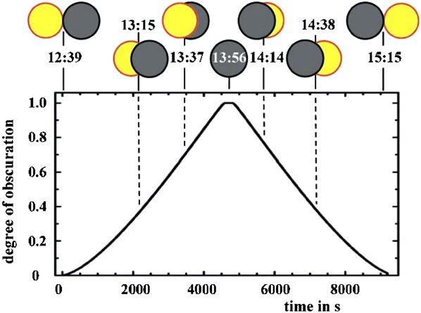
1300 K-P Möllmann and M Vollmer
weather conditions with a clear sky during more than 90% of the duration of the eclipse.
Since the illuminance measurements during the partial eclipse were nearly undisturbed by
clouds, it was tempting to have a detailed comparison to theoretical predictions. Surprisingly,
it has not been possible for us so far to find literature in textbooks [1–3] or, e.g., the best
available website on eclipses [5] on the problem of theoretically modelling illuminance during
the partial eclipse phase although this is probably common knowledge for astronomers and
buried in the old literature. Original publications of the last few decades usually focus on sky
brightness or radiance (rather than illuminance) as well as polarization, in particular during
the short period of totality, on predictions and on the influence on twilight and horizon colours
during totality [6–13]. The closest statement [6] to illuminance during the partial phase in
these papers was that the sky light may be considered as attenuated sunlight up to at least
99.8% obscuration.
Didactical papers on solar eclipses mostly deal with descriptions of the expected
phenomena and hints for observers, e.g., concerning photography. They are usually published
slightly ahead of an easily observable solar eclipse in Europe or America as was done in 1991,
1999 and 2006 in journals such as The Physics Teacher, Physics Education or other science
journals. In all cases, however, there was never an attempt to relate measured illuminances
to theoretical models although the latter are accessible with school mathematics. The only
exceptions are PC supported experiments on eclipses in binary star systems [14, 15].
In this paper, we present a simple geometrical model for the measured illuminance during
the partial phase of an eclipse. A comparison to the measurements gives a very good agreement.
We will not deal with illuminance or sky brightness during totality, where multiply scattered
light from outside the umbral region must be considered.
First, the conditions and experimental data of the recent eclipse will be presented.
Second, the theoretical model which is easily implemented in an introductory physics or
astronomy course—e.g. as an exercise—is developed. Third, the model is extended to describe
illuminance changes during arbitrary partial, total or annular eclipse. Finally, after a discussion
of a comparison of measurement and theory, predictions for the illuminance of other total,
annular or partial eclipse are discussed.
2. Measurements
2.1. Location of the 2006 eclipse
Figure 1 depicts all total solar eclipses from 2001 to 2025. Obviously, the eclipse of 29 March
2006 was the last total solar eclipse close to Central Europe for years to come. It started in
the Atlantic Ocean, then passed over Africa, parts of the Mediterranean before crossing over
Turkey into Asia. The duration of totality was more than 4 min in Africa and about 3 min and
45 s when it reached the coast of Turkey close to Antalya.
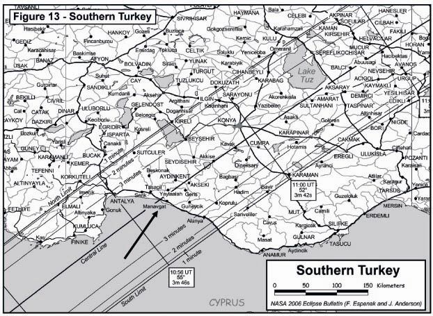
Figure 2 gives an extended view from the region in Southern Turkey, where totality lasted
for about 3 min and 45 s. Measurements were recorded at the beach near the city of Manavgat
which was very close to the central line.
The date of the eclipse had excellent weather predictions and fortunately, the sky during
the eclipse was nearly cloudless close to the beach. Overall, the disk of the sun was only once
slightly covered by very thin cirrus clouds near the end of the second partial phase.
2.2. Measuring illuminance
Illuminance is usually measured by calibrated equipment. The principle set-up is shown in
figure 3. The detector area must be oriented perpendicular to the light, which can be done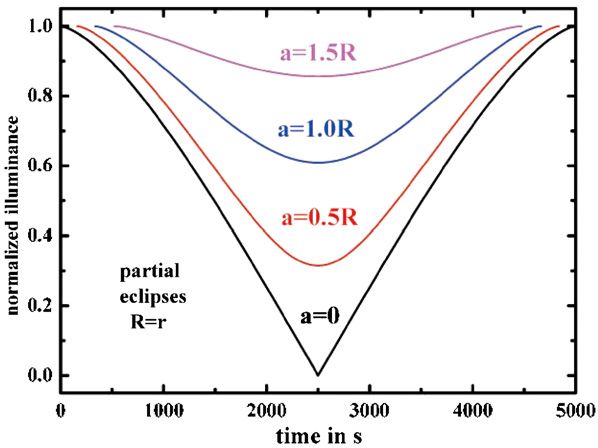
Measurements and predictions of the illuminance during a solar eclipse                                    1301

                              60°N

                   latitude
                              30°N

                                0°

                              30°S

                              60°S

                               180°W   120°W         60°W           0°        60°O        120°O         180°O
                                                                  longitude

                  Figure 1. Survey of the paths of all total solar eclipses in the period between 2001 and 2025
                  (after [5]).

                  Figure 2. Path of totality of the eclipse of 29 March 2006. The arrow indicates the city of
                  Manavgat, where measurements were recorded (after [5]).

easily by sticking some object perpendicular to it; its shadow must vanish. The instrument
was oriented each time directly before data were recorded with the exception of the first 3 min
after totality, where data were taken with the same orientation for every 5 to 10 s.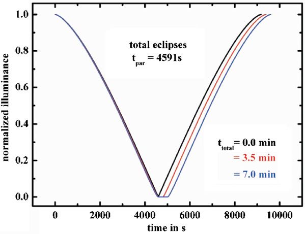
1302                                                                                   K-P Möllmann and M Vollmer

               Figure 3. Experimental set-up for measuring illuminance of sunlight during an eclipse.

               Figure 4. Measured illuminance during solar eclipse of 29 March 2006 near Manavgat/Turkey on
               a linear (left) and logarithmic (right) scale. The lines are no fit, but should just guide the eye.

      We used a battery operated digital Mavolux (Gossen) which can cover the illuminance
range from 0.1 lx up to 199 999 lx. The absolute accuracy of the instrument is given as 2.5%.
Systematic measurement errors can occur due to the cosine factor, i.e. if the incident light
is not propagating perpendicular to the detector area (see figure 3). Allowing for deviation
angle α of 2◦ , 5◦ , 10◦ or 20◦ would only result in recorded illuminance of 99.94%, 99.62%,
98.48 or 93.97%, respectively. Since during the eclipse measurements—for the sake of simple
transportable equipment—all adjustments were coarse and done manually, it may be possible
that deviation angles of a few degrees were present. However, even if α < 20◦ , which seems
to be a very large upper limit, the maximum systematic measurement errors are expected to
be around −6.0%. Read-out errors refer to the last digit and (with the exception of totality)
amount to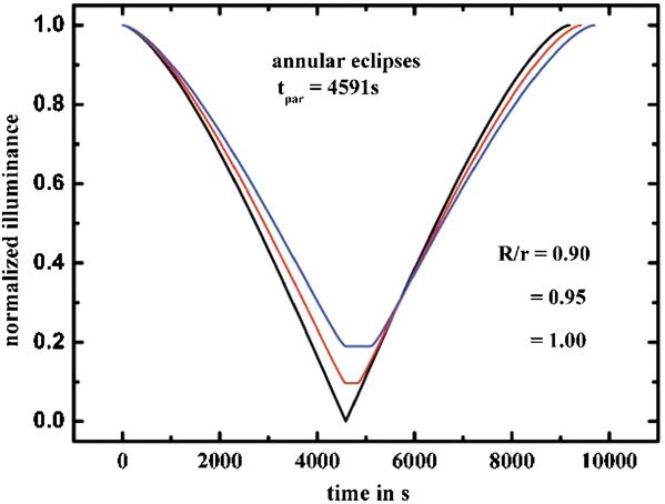
Measurements and predictions of the illuminance during a solar eclipse                                      1303

                  Table 1. Measured illuminance data as a function of time.
                  Time in s after start   Illuminance in lux   Time in s after start   Illuminance in lux
                    30                    111 800              4880                        870
                   390                    109 900              4890                      1030
                   750                    104 700              4900                      1261
                   930                    101 400              4910                      1432
                  1110                     98 100              4920                      1608
                  1290                     94 100              4930                      1815
                  1470                     89 700              4940                      1973
                  1650                     85 100              4950                      2200
                  1830                     80 000              4960                      2460
                  2010                     76 100              4970                      2650
                  2190                     70 700              4980                      2850
                  2370                     65 300              4990                      3060
                  2550                     59 200              5000                      3270
                  2730                     53 900              5010                      3500
                  2910                     47 600              5020                      3700
                  3090                     42 000              5030                      3980
                  3270                     36 900              5040                      4380
                  3450                     30 800              5050                      4600
                  3570                     26 800              5060                      4840
                  3630                     24 700              5250                      7780
                  3810                     19 200              5310                      9410
                  3990                     13 900              5370                     12 350
                  4170                      9300               5430                     13 700
                  4290                      6200               5610                     19 180
                  4350                      4600               5910                     29 600
                  4410                      3400               6090                     34 700
                  4470                      2200               6270                     42 000
                  4530                      1400               6570                     52 400
                  4598                          5              6690                     56 200
                  4710                          5              6990                     63 500
                  4810                          6              7170                     70 500
                  4820                         50              7590                     82 300
                  4825                        116              7770                     87 500
                  4835                        228              7950                     92 600
                  4840                        343              8130                     96 400
                  4850                        447              8970                    112 500
                  4860                        570              9390                    113 000
                  4870                        719

the sky, and any changes due to changing air mass with sun elevation [16] during the eclipse
were negligible.
     Maximum illuminance values increased from about 112 000 lx prior to 113 000 lx after
the eclipse. These values are typical for sea-level measurements with clear skies around noon
time [17]. As expected, the illuminance curves reveal a rather symmetric shape for both
partial phases. At first glance, the decrease from beginning to totality seems to be nearly
linear. However, a closer look reveals a complex shape (see section 3). During totality, the
background illuminance of about 5 to 6 lx is dominated by multiply scattered light from outside
the umbral region [6]. It usually shows asymmetric behaviour, which we did not investigate
any further due to our manual technique of data recording; we did record only three data points
during totality. The first few minutes directly after totality were measured in 5 to 10 s intervals
and revealed an increase in illuminance by a factor of 10 in the first 10 s and more than a factor
of 100 within the first minute.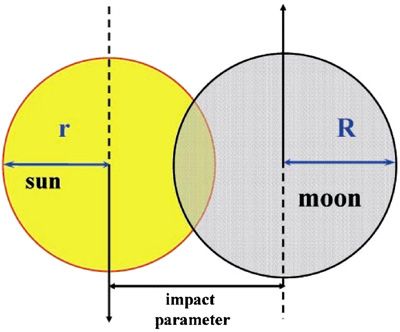
1304                                                                                  K-P Möllmann and M Vollmer

                  Figure 5. Scheme for modelling the solar eclipse: illuminance is proportional to the unobscured
                  area of the disk of the sun.

                  Table 2. Typical illuminances.

Full moon                                           Approximately 0.25 lx
Limit for colour vision                             Approximately 3 lx
Street lights                                       1–16 lx
Living room lights                                  120 lx
Good working room conditions                        1000 lx
Overcast sky                                        Order of 10 000 lx (depends on sun elevation + cloud thickness)
Cloudless sky, direct sun, summer                  >70 000 lx (depends on sun elevation)

     During the disturbance by cirrus clouds close to the end of the second partial phase,
illuminance was fluctuating in the indicated range. These values were not used for the later
comparison between experiment and theory.
     In order to have reference values, table 2 gives typical illuminance values for certain
well-known conditions. The illuminance for direct sunlight for a cloudless sky varies strongly,
depending on the optical air mass [16]. The given value 70 000 lx is a typical lower limit.
Outside of the atmosphere, it can reach values of about 140 000 lx [17].

3. Theoretical model for illuminance during the partial eclipse

3.1. Basic idea of the model

The principal idea for a theoretical modelling is illustrated in figure 5. It assumes that the
illuminance is directly proportional to the unobscured area of the disk of the sun.
     The measured illuminance is, of course, due to two contributions, direct sunlight and
skylight, which is either singly or multiply scattered sunlight [17]. The skylight brightness
varies as a function of the distance from the sun as many investigations have shown [17, 18].
This has, however, no influence on illuminance measurements since the sun is high in the
sky during the eclipse, and the detector is always oriented towards the sky centred around
the sun. Experimentally, the two illuminance contributions are easily found by recording two
measurements, the first one including all contributions (as was done for the eclipse) and the
second one, for which the direct sunlight is blocked off by an object which only covers a
small portion of the solid angle contributing to the skylight. The relative skylight contribution
varies according to the content of scatterers in the atmosphere. For clear skies around noon,
it typically amounts to between 10 and 20% of the direct sunlight contribution; for hazy skies
more than 30% is possible.
     Based on the theory of extended light sources, it is obvious that the direct sunlight
contribution is proportional to the unobscured area of the disk of the sun. A similar statement,
however, also holds for the skylight [6] which may be considered as attenuated sunlight up
to at least 99.8% obscuration. In the present case, the remaining 0.2% correspond to a time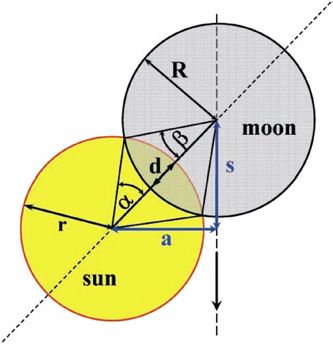
Measurements and predictions of the illuminance during a solar eclipse                     1305

interval of 10 s, i.e. the model should work quite well with the exception of a few seconds
around totality.
     The eclipse is modelled by letting the opaque and dark new moon cover part of the sun’s
disk. The eclipse starts when both disks are touching and totality occurs for 100% covering
of the sun. The duration of totality depends on the relative size of the disks of sun and moon
and their relative velocity. The theoretical model calculates the unobscured area of the sun as
a function of coverage, which is related to time.

3.2. Model assumptions and input parameters

In order to model the measured illuminance data, some simplifying assumptions are made in
order to address the problem at school and undergraduate university course level.
  • The sun and moon are treated as disks which are assumed to have an exactly spherical
    shape. This assumption neglects any limb effects, e.g. of lunar mountains, which give rise
    to the diamond ring effect during the last few seconds before totality. It also neglects any
    effects of prominences. For the present observation, this seems justified since prominences
    usually depend on sun spot activity and go along with observations of the red Balmer
    line rim regions of the sun during totality. During the last European eclipse of 11 August
    1999, there were many sun spots and easily observable red light due to prominences close
    to the rim. However, the 2006 eclipse was occurring close to a sun spot minimum, and
    naked eye observations were not quite successful in seeing any red light prominences.
    Hence, we conclude that prominences close to the rim did not have an influence on our
    measurements. Overall, the assumption of the exact spherical shape therefore seems not
    to be a severe restriction. It should hold with the exception of the last few seconds around
    totality, i.e. for nearly all of the partial phase of the eclipse, which is treated here.
  • For simplicity, the trajectories of sun and moon were considered to be straight lines rather
    than actual curved paths. This again is not a severe restriction, since comparison can be
    made according to the degree of coverage, which is independent of the type of motion. If
    necessary, the model could be extended to predefined trajectories.
  • The relative velocity of sun and moon was assumed to be constant. Again, this assumption
    is nearly fulfilled, since the duration of the eclipse is short compared to the time scales,
    required for the earth and moon on their elliptic paths around the sun and earth to
    appreciably change their velocities.
  • The brightness of the sun’s disk is assumed to be homogeneous which means that any
    effects due to prominences and sun spots are neglected. Again, this assumption is quite
    reasonable for the 2006 eclipse due to the very low activity of the sun.
    In order to calculate the illuminance for any type of eclipse, several input parameters have
to be chosen, namely the duration of the eclipse, the duration of totality or annularity, the
impact parameter and the sizes of the sun and moon.
  • The duration of the eclipse as well as of totality on the central line is usually known.
    These and many other eclipse data have been calculated for hundreds of eclipses of the
    past and the future [5].
  • The most simple case for an eclipse refers to being on the central line. In this case, the
    trajectories, fixed in the centre of the sun and moon, would be collinear. For all other
    cases, the trajectories will be parallel with an impact parameter which is the minimum
    distance between the centres of the sun and moon during the eclipse (figure 6).
  • The apparent sizes of the sun and moon depend on the distance between the sun and earth
    as well as on the one between the earth and moon. Obviously, their values depend on the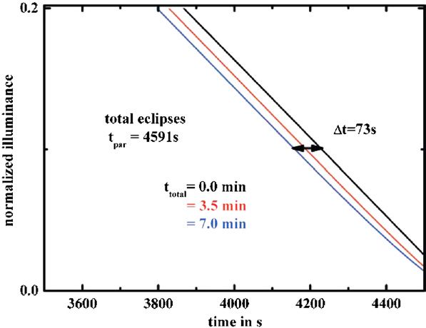
1306                                                                               K-P Möllmann and M Vollmer

               Figure 6. Geometry of the projected disks of the sun and moon during a partial eclipse. The
               arrows indicate the directions of the motions.

               Figure 7. Geometry for calculating the degree of obscuration during a solar eclipse.

    locations of earth and moon on their elliptic paths in space. The angular size of the moon
    may vary between the limits 29 22 and 33 30 (due to variations of earth–moon distance
    between 356 410 km and 406 740 km) and the respective values for the sun vary between
    31 32 and 32 36 (due to variations of earth–sun distance between 147 100 000 km and
    152 100 000 km).
  • Due to variations in the observed size, the angular diameter of the moon can be at maximum
    1.062 times the angular diameter of the sun, producing the longest total eclipse of 7 min
    and 31 s. Similarly, the angular diameter of the sun can be at maximum 1.11 times the
    angular diameter of the moon (i.e. moon diameter/sun diameter = 0.90), producing the
    longest annular eclipse of 12 min and 30 s.
  • For the purpose of our model, we deal with apparent radii and distances, which are given
    as dimensionless numbers with respect to the angular radius R of the moon. Hence,
    variations of the sun radius occur within an interval of 0.90 R to 1.062 R.

3.3. Theoretical model for illuminance during solar eclipses

In order to easily understand the theoretical model, we will first describe the situation for an
arbitrary obscuration. Then, the relative motion of sun and moon as a function of time is
connected to the degree of obscuration to give the illuminance as a function of time.

3.3.1. Degree of obscuration and illuminance.   Figure 7 depicts the geometry: the area of the
sun is partially covered by the moon. The two centres lie on the interrupted line. This situation
corresponds to a certain moment in time during an arbitrary eclipse. The relevant parameters
are radius r of sun, radius R of moon, angles α and β of the centres to the points where the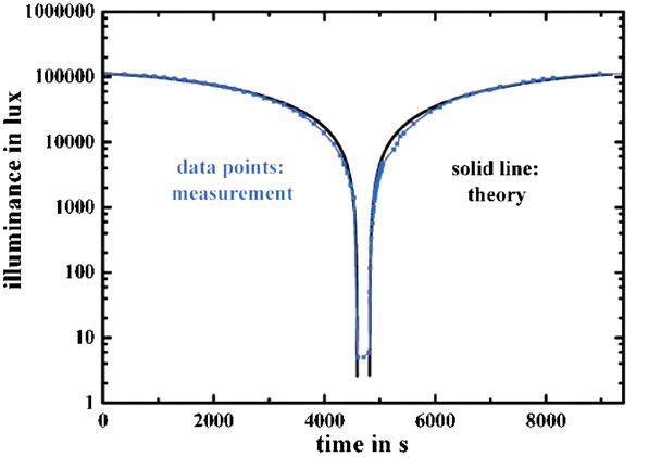
Measurements and predictions of the illuminance during a solar eclipse                              1307

                                                B
                                       r
                                       α
                               M                    D

                                                        E
                                                C

                  Figure 8. Expanded view of the portion of the sun which is covered by the moon.

                          r                     R

                          α                 β
                                   d

                  Figure 9. Expanded view of figure 7, defining the angles α and β.

perimeters cross each other and the distance d of the sun along the line of movement, which
is already covered.
     Obviously, the degree of obscuration p is given by the ratio of the sun’s area, which
is covered by the moon Acov (this corresponds to the shaded area, where the distance d is
indicated), to the sun’s area Asun = π r2. The major problem consists in calculating Acov.
According to the expanded view in figure 8, Acov is composed of two parts with different forms
(two shaded areas) since the radii r and R of the boundary lines are generally different.
     The shaded area in the right, determined by BECDB is given by the area r2 × α of the
segment of the circle (MBDCM) minus the area of the triangle (MBCM). The latter is twice
the area of the triangle (MEBM), which is the product (r × cos α) × (r × sin α). Hence, the
shaded area (BECDB) is given by r2 × (α − cos α × sin α).
     Similarly, the other shaded area is given by R2 × (β − cos β × sin β).
     The only remaining problem is to calculate the angles α and β as a function of r, R
and d.
     According to figure 9, cos α and cos β can be computed using the law of cosines in the
shown triangle. One finds, e.g.,
                  R 2 = r 2 + (R + r − d)2 − 2r(R + r − d) cos α,                                    (1)
which gives

                           1 r 2 − R 2 + (R + r − d)2
                   cos α =                                 .                                  (2)
                           2       r · (R + r − d)
A very similar relation holds for cos β such that we can write the final result for the degree of
obscuration p as
                     r 2 (α − sin α · cos α) + R 2 (β − sin β · cos β)
               p=                                                                             (3)
                                            πr2
with

         1 r 2 − R 2 + (R + r − d)2                                 1 R 2 − r 2 + (R + r − d)2
cos α =                                         and       cos β =                               .
         2        r · (R + r − d)                                   2     R · (R + r − d)
                                                                                              (4)
1308                                                                             K-P Möllmann and M Vollmer

                Figure 10. Geometry for an arbitrary eclipse, occurring for impact parameter a between the sun
                and moon.

The normalized measured illuminance L/Lmax. is then given by
                 L
                     = 1 − p.                                                                             (5)
                Lmax
In the following, examples for the obscuration due to total, partial and annular solar eclipses
will be treated (we neglect hybrid eclipses where along certain portions of the path, the eclipse
is total and for other portions it is annular).

3.3.2. Relating obscuration to specific parameters of an eclipse.    The geometry of figure 7
does not yet include the movement of sun and moon. For simplicity, we will keep the sun fixed
and let the moon move alone. Figure 10 shows the most general geometry which, compared
to figure 7, is rotated. The sun is kept fixed and the moon moves from top to bottom along the
vertical direction. From figure 10, it is obvious that the impact parameter a is the minimum
distance that the centres of sun and moon can have, which occurs for greatest obscuration
when the distance s is zero. The impact parameter a as well as the radii r and R of sun and
moon defines the type of eclipse.
     From the law of Pythagoras for the rectangular triangle, it follows that (r + R − d)2 =
a + s 2 ; hence,
  2

                               √
                 d = r + R − a2 + s 2.                                                     (6)

Any particular distance x which is traversed in time t along the moon’s trajectory can be easily
described as x = v × t, where v is the relative velocity between the sun and moon. The latter
is related to the period tpar of the eclipse from the first contact to the start of totality or from
the first contact to the last contact tall.
     In figure 10, the first contact would correspond to a situation where the moon would just
touch the sun at a distance s0 above the horizontal line (defined by a). Due to symmetry, the
last contact would correspond to a similar distance s0 below the horizontal line. The total
distance travelled between the first and last contacts is then given by 2s0. Obviously, the
velocity v is given by
                     2s0                          s0
                v=               or        v=         .                                                   (7)
                     tall                        tpar
Measurements and predictions of the illuminance during a solar eclipse 1309
We now consider the change of s from the first contact to maximum obscuration. Moving
with constant velocity v along the vertical direction, the distance s as a function of time from
the first contact to totality decreases from s0 to zero according to
t
s(t) = s0 1 − . (8)
tpar
Now, all equations are given, which are needed to calculate the illuminance of any given
eclipse during the partial phases. Inserting s(t) from equation (8) into equation (6) gives d(t),
which is needed to compute cos α and cos β equation (4)). The latter are used to compute the
degree of obscuration p (equation (3)) and the normalized illuminance (equation (5)).
The above equations have
3.3.3. Specific conditions for partial, total and annular eclipses.
been used to produce xls-files, which calculate the degree of obscuration and normalized
illuminances. The input parameters of these files are
• radius of sun r and radius of moon R; usually only the dimensionless ratio R/r is used,
• the impact parameter a is usually also given as dimensionless units a/r,
• either the time from the first contact to maximum obscuration tpar or the total time tall of
the eclipse,
• for total eclipses also the time of totality ttotal,
• for annular eclipses, the times t12 between first and second and t23 between second and
third contacts (the four contacts are defined by any apparent touching of the perimeters of
the sun and moon).
The most general case of an eclipse is a partial eclipse. It is defined by 0 < a < r + R.
A total eclipse is defined as a special case of a partial eclipse for a = 0 if R > r. Here,
illuminance is calculated from the first contact to totality. During totality, p is set to unity and
illuminance to zero. During the second partial phase, degree of obscuration and illuminance
are symmetrical to the first partial phase. A total eclipse does also easily allow to calculate
the ratio of the radii of the sun and moon since
R ttotal
=1+ . (9)
r tpar
An annular eclipse is treated similar to the total eclipse; however, R/r < 1. Again, the ratio
of the radii of the sun and moon is connected to the respective times. If t12 denotes the time
between first and second contacts and t23 denotes the time between second and third contacts
(while the moon is travelling in front of the disk of the sun), one finds
R t12
= . (10)
r t12 + t23
3.3.4. Example for the most simple analytical solution. The above equations allow to compute
the degree of obscuration and illuminance for any eclipse. This procedure works easily with
computer programs like Excel or Origin etc; however, there is also one very simple analytical
solution available. For r = R, and for a location on the central line (a = 0), this corresponds
to a duration of totality of zero; one immediately sees that α = β and therefore
2(α − sin α · cos α)
p= . (11)
π
From equation (6), the distance d(t) = 2R − s(t) and from equation (8), s(t) = s0 ×
(1 − t/tpar) = 2R × (1 − t/tpar); hence,
d(t) = 2R × (t/tpar ). (12)1310 K-P Möllmann and M Vollmer
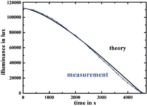
Figure 11. Modelled degree of obscuration of the sun as a function of time during the eclipse of
29 March 2006.
As expected, equation (12) gives the initial condition d = 0 at the start at t = 0 and d = 2R at
the moment of totality at t = tpar. Inserting d into equation (4) leads to cos α = (1 − t/tpar ),
and equations (5) and (11) finally give
2
2 t t t t . (13)
L = Lmax . · 1 − · arccos 1 − − 1− · 2 −
π tpar tpar tpar tpar
Equation (13) has the advantage that it gives the illuminance analytically as a function of
time t from the start of the eclipse until totality. The second partial phase will be symmetric.
4. A comparison of measurement and theory
The experimental data from figure 4 have been compared to the theoretical prediction. The
input parameters for the model were ttotal = 224 s, tpar = 4591 s, giving R/r = 1.0488. This may
only apply to the data within several per cent since the exact location of the beach, where data
were taken, was not precisely determined; it was a few kilometres distant from the central line,
thereby slightly decreasing both times by a few seconds. Figure 11 gives the computed degree
of obscuration p as a function of time after the start of the eclipse. On top, the obscuration of
the sun by the moon is indicated for several times.
A direct comparison of measured illuminance during the first partial phase with this
model is shown in figure 12. After the second partial phase, the illuminance was slightly
higher than that before the eclipse. This increasing trend could be accounted for in a more
thorough analysis, which was, however, not performed here, since the overall deviations due
to experimental errors and theoretical uncertainties are anyhow expected to be around several
per cent. In the first partial phase, most experimental data are slightly below theory as was
expected from the systematic error due to the manual alignment. Figure 13 depicts the same
data and theory for the whole eclipse with a logarithmic scale in order to better visualize the
huge decrease in illuminance by more than a factor of 20 000 during the eclipse. The overall
agreement is very good.Measurements and predictions of the illuminance during a solar eclipse 1311
Figure 12. A comparison of data from the 2006 eclipse and theory on a linear scale.
Figure 13. A comparison of data from the 2006 eclipse and theory on a log scale.
5. Application of the model to other eclipses and limitations
The model for the illuminance during solar eclipses can be easily applied to other total eclipses
as well as annular and partial eclipses. Figures 14 and 15 depict results for total eclipses (which
for the sake of simplicity had the same tpar = 4591 s as the eclipse in March 2006) with different
durations of totality. ttotal = 0.0 min corresponds to a hybrid eclipse which just reaches totality
at one point on earth. At first glance, all three illuminance curves look the same; however, the
larger the radius of the moon, the faster the drop of illuminance. For example, the eclipse with
7 min totality has reached the 10% level of illuminance already 73 s earlier than the hybrid
eclipse (see figure 15).
Figure 16 depicts three different annular eclipses. Again, tpar was arbitrarily chosen to be
4591 s. Decreasing the apparent size of the moon by 5% and 10% does not not only lead to a
faster drop in illuminance, but also lead to residual illuminances of 10% and 20%, respectively.
Finally, figure 17 gives examples for the illuminance of partial eclipses. Partial eclipses
can be observed much more often. The figure depicts normalized illuminances for R = r and1312 K-P Möllmann and M Vollmer
Figure 14. A comparison of predicted normalized illuminances for several total eclipses.
Figure 15. Expanded view of figure 14, showing the differences between the eclipses.
several impact parameters. In the case of a = R, for example, the rim of the moon would just
touch the centre of the sun’s disk at the greatest obscuration of about 39%, giving rise to a
normalized illuminance of about 61%. The same effect could normally result if some clouds
were blocking direct illumination by the sun. This may also explain why many people do not
note a partial eclipse from illuminance changes alone.
One word of caution: a comparison of ttotal and tpar in figure 14 as well as from the actual
data of very long total eclipses (e.g. the 1991 eclipse in Mexico with 6 min and 53 s) would lead
to ratios of radii above 1.062 when using equation (9). Similar problems occur for the very
long annular eclipses. This shows the limitations of our model due to the model assumptions,
in particular the straight motion rather than the actual curved trajectories. Of course, this
model shall give a first explanation of the measured illuminance curves as may be treated in
undergraduate courses. For this purpose, it is still possible to draw reasonably quantitative
conclusions from figures 14 to 17. If, however, very high precision is required, the model
should be extended by using realistic curved trajectories.Measurements and predictions of the illuminance during a solar eclipse 1313
Figure 16. Normalized illuminances for several annular eclipses.
Figure 17. Normalized illuminances for several partial eclipses.
6. Conclusions
Measurements of illuminance during the partial phase of a solar eclipse have been compared
to theoretical predictions, based on a geometrical model which applies to all types of eclipses,
partial, annular and total. The comparison showed a very good agreement, regarding the
crude measurement with manual adjustments. The model is simple enough to be treated in
undergraduate physics courses or at school level. Its practical use is, unfortunately, limited
to the rather rare events of solar eclipses. Figure 1 gave a survey of total solar eclipses until
2025; a similar graph for annular eclipses and other graphs and data for the more distant future
are available [5].
Obviously, there are some chances to observe total eclipses and measure illuminances in
the near future; however, Europeans must travel quite far at least for totality. Besides the one
of 1 August 2008 and disregarding any weather predictions, the best choice for the near future
is the eclipse of 22 July 2009, which can be observed mostly in India (in the morning hours1314 K-P Möllmann and M Vollmer
with low sun) and China. It belongs to the eclipse family of Saros 136 and is the sequel of
the eclipse of 1991 in Hawaii. It will last a near record of 6 min and 39 s. After this one, the
next really good chance will probably be the sequel of the 1999 European eclipse which will
happen in August 2017 all across the United States. Still a long time to go, but definitely worth
to go for them not only for doing measurements, but just to enjoy one of the most spectacular
phenomena of mother nature.
Acknowledgment
We wish to thank Steffen Möllmann for helpful discussions.
References
[1] Littmann M and Willcox K 1991 Totality: Eclipses of the Sun (Honolulu: University of Hawaii Press) new
edition includes Fred Espanak as coauthor, see [5]
[2] Maunder M and Moore P 1998 The sun in Eclipse (Berlin: Springer)
[3] Harrington P S 1997 Eclipse (New York: Wiley)
[4] Vollmer M and Möllmann K-P 2006 Total eclipse aficionados seek out the best observation spots Phys. Educ.
41 193–5
[5] http://sunearth.gsfc.nasa.gov/eclipse/eclipse.html
[6] Sharp W E, Silverman S M and Lloyd J W F 1971 Summary of sky brightness measurements during eclipses
of the sun Appl. Opt. 10 1207–10
[7] Shaw G E 1975 Sky brightness and polarization during the 1973 African eclipse Appl. Opt. 14 388–94
[8] Gedzelman S D 1975 Sky color near the horizon during a total solar eclipse Appl. Opt. 14 2831–7
[9] Silverman S M and Mullen E G 1975 Sky brightness during eclipses Appl. Opt. 14 2838–43
[10] Shaw G E 1978 Sky radiance during a total solar eclipse: a theoretical model Appl. Opt. 17 272–6
[11] Mottmann J 1980 Solar eclipse predictions Am. J. Phys. 48 626–8
[12] Können G P 1987 Skylight polarization during a total solar eclipse: a quantitative model J. Opt. Soc. Am. A4
601–8
[13] Geyer E H, Hoffmann M and Volland H 1994 Influence of a solar eclipse on twilight Appl. Opt. 33 4614–9
[14] Williams G 2005 Binary-star eclipse simulated with PC drawing package Phys. Educ. 40 124–5
[15] http://instruct1.cit.cornell.edu/courses/astro101/java/eclipse/eclipse.htm
[16] Vollmer M and Gedzelman S 2006 Colors of the sun and moon: the role of the optical air mass Eur. J. Phys.
27 299–309
[17] Tousey R and Hulburt E O 1947 Brightness and polarization of the daylight sky at various altitudes above sea
level J. Opt. Soc. Am. 37 78–92
[18] Hulbert E O 1952 Explanation of the brightness and color of the sky, particularly the twilight sky J. Opt. Soc.
Am. 43 113–8You can also read