Description of the CO2 inversion production chain 2020 - version 1.0 Issued by: CEA
←
→
Page content transcription
If your browser does not render page correctly, please read the page content below
ECMWF COPERNICUS REPORT

Copernicus Atmosphere Monitoring Service

                Description of the CO 2 inversion
                production chain 2020
                version 1.0

                Issued by: CEA
                Date: 27/04/2020
                Ref: CAMS73_2018SC2_ D5.2.1-2020_202004_ CO2 inversion production chain_v1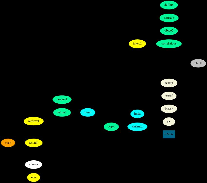
This document has been produced in the context of the Copernicus Atmosphere Monitoring Service (CAMS).
The activities leading to these results have been contracted by the European Centre for Medium-Range Weather Forecasts,
operator of CAMS on behalf of the European Union (Delegation Agreement signed on 11/11/2014). All information in this
document is provided "as is" and no guarantee or warranty is given that the information is fit for any particular purpose.
The user thereof uses the information at its sole risk and liability. For the avoidance of all doubts, the European Commission
and the European Centre for Medium-Range Weather Forecasts has no liability in respect of this document, which is merely
representing the authors view.
Copernicus Atmosphere Monitoring Service

                    Contributors

                    CEA
                    Frédéric Chevallier

CAMS73_2018SC2_ D5.2.1-2020_202004_ CO2 inversion production chain_v1   Page 3 of 15
Copernicus Atmosphere Monitoring Service Table of Contents 1. Preprocessing 5 1.1 Data collection 5 1.2 Update of the atmospheric mass fluxes 6 1.3 Update of the auxiliary files 6 1.4 Preliminary forward transport simulation 6 2. Method 7 3. Parallelization 8 4. Code 9 5. Outputs 10 6. Post-processing 12 7. Help desk 13 8. References 14 CAMS73_2018SC2_ D5.2.1-2020_202004_ CO2 inversion production chain_v1 Page 4 of 15
Copernicus Atmosphere Monitoring Service

Introduction
The inversion system that generates the CAMS global CO2 atmospheric inversion product is called
PYVAR. It has been initiated, developed and maintained at CEA/LSCE within the series of precursor
projects GEMS/MACC/MACC-II/MACC-III. This document presents its main features and the
production chain that goes through it.

1. Preprocessing
Each product release necessitates a series of preparatory steps before the inversion scheme PYVAR
is run. They are described hereafter.

1.1 Data collection

Atmospheric measurements are primarily collected from four large living databases:

    •   the     NOAA        Earth      System Research    Laboratory    Observation    Package
        (https://www.esrl.noaa.gov/gmd/ccgg/obspack/),
    •   the World Data Centre for Greenhouse Gases archive (WDCGG,
        http://ds.data.jma.go.jp/gmd/wdcgg/),
    •   the Réseau Atmosphérique de Mesure des Composés à Effet de Serre database (RAMCES,
        http://www.lsce.ipsl.fr/),
    •   the Integrated Carbon Observation System- Atmospheric Thematic Center (ICOS-ATC,
        https://icos-atc.lsce.ipsl.fr/).

The collection for PYVAR is either automatic (by harvesting relevant http, ftp or directories) or
manual by directly contacting data providers. Once all databases have been updated, they are
manually checked for changes:

    •   changes in file names, that need to be reported in the site selection script and in subroutine
        obsco2.py of PYVAR,
    •   changes in file format, including units, that need to be reported in subroutine obsco2.py of
        PYVAR,
    •   changes in site availability or record length (sites with less than five years’ worth of data are
        not assimilated).

Then, the site selection script can be run. The site selection depends on the data provider (i.e. trust
in the quality of the data calibration), on the record length and on the performance of the transport
model used in PYVAR in simulating its variability. The script copies all selected files in a unique
directory that is stamped with the release identifier.

Since year 2019, CAMS has also been producing atmospheric inversions based on satellite retrievals
from the second Orbiting Carbon Observatory (OCO-2, https://oco.jpl.nasa.gov/oco-2-data-center/).

CAMS73_2018SC2_ D5.2.1-2020_202004_ CO2 inversion production chain_v1                          Page 5 of 15
Copernicus Atmosphere Monitoring Service
1.2 Update of the atmospheric mass fluxes
Any extension of the assimilation period forward in time requires corresponding atmospheric mass
fluxes from the LMDZ global atmospheric transport model, nudged towards ECMWF horizontal winds.
The reference simulation of the full LMDZ model is done on one of the supercomputers of TGCC
(http://www-hpc.cea.fr/fr/complexe/tgcc.htm). The mass flux files (phystoke.*, flustoke.* and
flustokev.*) that it generates are saved on tapes for reference and then distributed on relevant active
directories for use by the off-line version of LMDZ within PYVAR.
1.3 Update of the auxiliary files
In addition to the mass flux files, some time-dependent input files of PYVAR have to be updated at
least once a year. Those are:
• annual fossil fuel fluxes1, that combine Emissions Database for Global Atmospheric Research
gridded distributions (EDGAR, http://edgar.jrc.ec.europa.eu/) and the most recent Carbon
Dioxide Information Analysis Center annual global totals (http://cdiac.ornl.gov/GCP/),
• 3-hourly fire emission fluxes 2 from the Global Fire Emissions Database (GFED,
http://www.globalfiredata.org/), and CAMS’s Global Fire Assimilation System (GFAS,
http://atmosphere.copernicus.eu/) for the recent months not yet available in GFED,
• monthly sea ice cover from ERA5,
• monthly prior ocean fluxes from the Copernicus Marine Environment Monitoring Service
(CMEMS, https://marine.copernicus.eu/).
3-hourly prior fluxes from undisturbed vegetation are climatological in PYVAR and are therefore
usually not updated.
1.4 Preliminary forward transport simulation
A preliminary simulation of the atmospheric transport is performed and compared to all surface
measurements that can be potentially assimilated for the period from 1979 to the most recent data
in order to:
• visually validate the above updates in the mass fluxes, in the auxiliary files and in the
observation interface,
• compute the statistics of the measurement high frequency variability (used as a proxy for
transport model errors, see §15 of Chevallier et al., 2010),
• remove measurement outliers (see §16 of Chevallier et al., 2010).
A second script multiplies the observation error standard deviation by the square root of the number
of local data within each day in order to neglect temporal error correlations in the inversion system
1
for the prior fluxes
2
for the prior fluxes
CAMS73_2018SC2_ D5.2.1-2020_202004_ CO2 inversion production chain_v1 Page 6 of 15Copernicus Atmosphere Monitoring Service
(see §15 of Chevallier et al., 2010). A last script averages consecutive measurements within a month
and adjusts the observation error standard deviation accordingly. After this stage, all selected
measurements are gathered in a single file (prev_monitor.txt) with necessary metadata (site name,
data provider, year, month, index of the transport model time step within the month, index of the
transport model 3D grid box, observation error standard deviation). They can then be assimilated.
For the satellite retrievals, in order to reduce the data volume without loss of information at the scale
of a global model, glint and nadir OCO-2 retrievals are averaged in 10-second bins following the
approach defined by the second Model Intercomparison Project (MIP-2) of OCO-2 (Crowell et al.,
2019). The retrieval averaging kernels, prior profiles and Bayesian uncertainty are accounted for in
the assimilation. The interpolation procedure between the model vertical grid and the retrieval grid
is described in Section 2.2 of Chevallier, 2015). Last, in order to account for likely correlations between
the transport model errors at the sub-grid scale, we de-weigh the binned retrievals that fall within a
same grid box for a same orbit by inflating the assigned error variance (σ2) by the number of retrievals
in the box.
2. Method
Given a vector of prior values of a series of state variables xb with an associated error covariance
matrix B, and given a vector of observations yo, with an associated error covariance matrix R, the
present scheme determines statistically optimum values of the state variables, xa. To do so under the
hypothesis of unbiased normally-distributed errors for xb and yo, it minimizes a cost-function which
measures the misfit to the background variables and to the observations:
J(x) = (x - xb)T B-1 (x - xb) + (H(x) - y)T R-1 (H(x) - yo)
where H is the observation operator (or forward model) that provides the model-equivalent of the
observations. H mostly consists in an atmospheric transport model. Note that R includes the error of
H in representing the measured variables.
The minimum of J(x) is found by an iterative process, and not by any analytical expression. At each
iteration, a descent direction is determined, using the value of the cost function gradient:
gradxJ(x) = 2 B-1 (x - xb) + 2 HT R-1 (H(x) - yo)
where HT is the adjoint operator of the Jacobian matrix H of H (i.e. {∂yi/ ∂xj}i,j).
In contrast to other formulations of the Bayesian estimation problem (analytical ones or ensemble
ones), the variational approach is limited in the dimension of neither x nor yo, provided B and R can
be inverted. This is the case for R because this matrix is taken as diagonal, following the usual practice
in atmospheric inversions. B includes off-diagonal terms (temporal and spatial correlations defined
by e-folding lengths), because it is expressed as the Kronecker product of the eigenvalue
decomposition of the two (spatial and temporal) correlation matrices, sandwiched with the vector of
prior error standard deviations.
CAMS73_2018SC2_ D5.2.1-2020_202004_ CO2 inversion production chain_v1 Page 7 of 15Copernicus Atmosphere Monitoring Service
For a better efficiency of the minimization of J(x), x is preconditioned with the eigenvectors of B,
which means that the minimization control variable is ζ= B-1/2 (x - xb) rather than x. Doing that, the
cost function J(x) remains unchanged, while its gradient can be written:
gradζJ(x) = 2 ζ + 2 B+1/2 HT R-1 (H(x) - yo)
The computation of B1/2 x is approximated by C1/2 x ◦ s., with C and s being, respectively, the
correlation matrix and the vector of standard deviations of B, and ◦ being the Hadamard product.
Further, C1/2 is approximated by U1/2 uT, with U and u the eigenvector and eigenvalue matrices of the
principal component analysis of C. Eigenvalues less than 0.5 are discarded because they are likely not
precise enough. These approximations are discussed by Thompson (2016).
The minimizer itself is either a limited memory quasi-Newton method, the M1QN3 software from
Gilbert and Lemaréchal (1989) or (systematically for CO2) the Lanczos version of the conjugate
gradient algorithm (Fisher 1998, Desroziers and Berre 2012).
Bayesian error statistics of xa (defined by the posterior error covariance matrix A) are computed from
a stochastic ensemble of inversions defined from the following two equations. These equations are
implemented in subroutine initco2.py.
xb = xt + WT w1/2 q
with an arbitrarily defined true value of x, q a vector of size the dimension of xb, which is a
xt
realization of random variables with standard normal distributions. W and w are the eigenvector and
eigenvalue matrices of the principal component analysis of B, so that B = WT w W.
y = yt + VT v1/2 p
with yt = H(xt), and V and v the eigenvector and eigenvalue matrices of the principal component
analysis of R, so that R = VT v V. Vector p is a vector of size the number of observations, which is a
realization of random variables with standard normal distributions.
The scientific detail of the software is given in Chevallier et al. (2005, 2007, 2010).
3. Parallelization
Most of the computing time of PYVAR is spent in transport model computations (operator H and its
tangent-linear – H – and adjoint – HT – versions). In order to minimize the computation wall-clock
time of the inversion, two levels of parallelization are used.
In the first one, the globe is split into a series of latitude bands (typically 7) that run on different cores
and communicate through Message Passing Interface (MPI) subroutines. For the purpose of
efficiency, these cores are usually all the cores of a same socket.
In the second one, the transport model is run in parallel overlapping temporal segments. One
segment typically covers a period from August until December of the following year (17 months) and
CAMS73_2018SC2_ D5.2.1-2020_202004_ CO2 inversion production chain_v1 Page 8 of 15Copernicus Atmosphere Monitoring Service overlaps with other segments from August until December of each year. This approach allows efficient embarrassingly parallel workload, i.e. tasks that do not need communicating, within each iteration step. The tracer increments and the adjoint sensitivities are carried out from one segment to the next through a global bias term. The simulation that provides the linearization point is only parallelized through MPI and does not use the bias-term simplification. This bias term assumes that all mole fraction increments are uniformly mixed in the global atmosphere. Unwanted side effects of this approximation are damped by the long overlap period and by the update of the linearization point during the minimization (in practice we perform two iterations of the outer loop, one of 20 iterations and a second of 50 iterations). At the highest level, the inversion manages all segments at once with a single cost function J(x). More details of this physical parallelization are given in Chevallier (2013). In the code, it is managed by subroutine enslmdz.py. The combination of the two parallelization levels allows a 40-year inversion to be run on 40 sockets, with a speed gain of more than two orders of magnitude compared to a computation on a single processor. Still, about a month of computation is needed to perform it at the resolution of the LMDZ model as it is currently used in PYVAR. 4. Code The code is written in Python language and its current version was tested with official Python releases 2.7.12. PYVAR also needs an atmospheric transport numerical model, LMDZ for CAMS. It is called in lmdz.py by a system call to the model executable. This documentation does not describe the transport numerical model. All routines of PYVAR are in the Tools directory, except main.py which is one directory level above. Figure 1 shows the dependencies between the files. PYVAR is run by typing: python main.py DEF In this command line, main.py is the driver routine and DEF is the directory of the configuration files co2.def, files.def and pyvar.def. Other files exist in this directory for other applications of PYVAR than CO2: they are not discussed here. Each configuration file is made of a series of 2-line statements, the first line describing the variable given in the second line. The line number of the variable (starting from zero according to the Python convention) appears in brackets in the legend line for reference in the PYVAR code. pyvar.def contains the PYVAR variables shared by the all applications, like the task to be performed by the software (inversion, passive observation monitoring, test adjoint, etc.). co2.def and gch.def contain the variables that are specific for the CO2 application. files.def contains the names of the files and directories used by PYVAR. CAMS73_2018SC2_ D5.2.1-2020_202004_ CO2 inversion production chain_v1 Page 9 of 15
Copernicus Atmosphere Monitoring Service

Figure 1. PYVAR subroutine tree. Only the modules are shown (i.e. the files *.py), rather than the individual
subroutines in each one of them. The extensions '.py' have been omitted for clarity. Boxes have been arbitrarily
displayed in space. The color code is the following: orange represents the driver routine; yellow, green, blue (cyan)
and beige indicate modules of increasing depth in the calling structure. obsco2 is both a level-1 and a level-2
module and is shown in green. ooper is both a level-1 and a level-2 module and is shown in green. simul is both a
level-2 and a level-3 module and is shown in blue (cyan). check is called in many places and is in grey. classes
defines Python classes and has been left blank. The rectangle box 'LMDz' refers to the executable of the transport
model.

During the program execution, the variables circulate through the state vector x, through the
preconditioned vector ζ and through the Python structure auxiliary (defined in Tools/classes.py) that
contains all variables that are not optimized (i.e. not in x) but that are required for the computation
of the cost function J(x).

5. Outputs
PYVAR has three main outputs. One is a log file, whose name is defined in line 17 of pyvar.def. The
log file contains the same information than that that given in the standard output. The second main
output file is called monitor.txt and is created in the execution directory (the execution directory is
defined in line 7 of pyvar.def) by module lmdz.py. monitor.txt is a text file with as many lines as there
are observations. Each line contains the following variables separated by spaces:

    •   observation identifier,
    •   observation date (yyyymm),

CAMS73_2018SC2_ D5.2.1-2020_202004_ CO2 inversion production chain_v1                                Page 10 of 15
Copernicus Atmosphere Monitoring Service
• observation time step with respect to the transport model,
• observation latitude index with respect to the transport model,
• observation longitude index with respect to the transport model,
• observation measurement value,
• prior equivalent of observation,
• posterior equivalent of observation,
• observation error,
• observation attribute (its definition varies with the observation type).
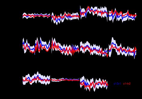
Figure 2. Summary diagnostics generated for each measurement site: the time series of the
measurements (in red, with the observation 1-sigma uncertainty) and of the posterior simulation (in
blue) are shown together with summary statistics of the misfits compared to the assigned observation
uncertainty. In this example, the measurements at station TKB in the suburb of Tokyo, Japan, have a
much larger variability than the model, even after the inversion. Further, the model after the
inversion is still biased by 3 ppm. Posterior biases at the other stations are usually less than 1 ppm
and reach 2.1 ppm at the maximum (station HPB). TKB has been consequently blacklisted
The last main output file is called monitor.nc or analysis.nc (depending on the task to run), and is also
created in the execution directory (by the module save.py). Depending on the configuration, it
contains some of the following maps at the resolution of the transport model:
• Obs${yyyymm}${dn}: monthly mean map of yo for month ${yyyymm}. For the project 'co2',
${dn} refers to daytime ('d') or night-time ('n'). For the other projects, ${dn} is void. The
horizontal grid comes from the transport model.
• FGobs${yyyymm}${dn}: same as Obs${yyyymm}${dn} for the first-guess-equivalent of
observations.
• ANobs${yyyymm}${dn}: same as Obs${yyyymm}${dn} for the posterior-equivalent of
observations.
• NBobs${yyyymm}${dn}: map of the number of observations for the above averages.
CAMS73_2018SC2_ D5.2.1-2020_202004_ CO2 inversion production chain_v1 Page 11 of 15Copernicus Atmosphere Monitoring Service
• BGv${var}${spec}_${yyyymmdd}: map xb. ${var} is the variable type: fluxes ('flux') or scaling
factors ('scale'). ${spec} is the species name. ${yyyymmdd} is the date. If the variable refers to
the initial time step, '_${yyyymmdd}' is omitted.
• BGe${var}${spec}_${yyyymmdd}: same as BGv${var}${spec}_${yyyymmdd}, but for the prior
error standard deviations of the fluxes.
• ANv${var}${spec}_${yyyymmdd}: same as BGv${var}${spec}_${yyyymmdd} but for xa.
• CLv${var}${spec}_${yyyymmdd}: if the option 'perturb prior' has been activated (in pyvar.def),
this variable contains the map of xt., in the same way than BGv${var}${spec}_${yyyymmdd}.
6. Post-processing
The quality control of the inversion relies on a series of verification procedures:
• Control of the log files, including the reduction of the cost function J(x) and of the norm of its
gradient gradζJ(x),
• Control of the misfits to the assimilated data (see the example of Fig. 2) and to independent
ones (aircraft and column retrievals, including in terms of mean latitudinal gradients, see the
example of Fig. 3),
• Control of the global, regional (Transcom-3) and national (for the largest countries and the
European Union) annual carbon budgets (see the example of Fig. 4).
Figure 3. Summary statistics of the misfits of the posterior simulation to dependent and independent
measurements. The boxes and whiskers are shown per measurement type. A benchmark inversion (Poor Man’s
inversion) allows defining skill for the inversion.
CAMS73_2018SC2_ D5.2.1-2020_202004_ CO2 inversion production chain_v1 Page 12 of 15Copernicus Atmosphere Monitoring Service The result of each verification procedure is compared to the result obtained for the previous release in order to detect possible anomalies. Once the verification procedures are finished, output files are reformatted and delivered to ECMWF. Figure 4. Time series of the inverted regional carbon budgets over land from 1979 until 2014 in two product releases. A positive flux is a flux to the atmosphere. Last, all preprocessing, PYVAR, postprocessing scripts and results are saved on tape under a unique identifier for future reference. 7. Help desk All queries about PYVAR or its products should be sent to copernicus-support@ecmwf.int. Acknowledgements The author is very grateful to the many people involved in the surface, aircraft and satellite CO2 measurements and in the archiving of these data that are kindly made available to him each year. CAMS73_2018SC2_ D5.2.1-2020_202004_ CO2 inversion production chain_v1 Page 13 of 15
Copernicus Atmosphere Monitoring Service

8. References
Chevallier, F., M. Fisher, P. Peylin, S. Serrar, P. Bousquet, F.-M. Bréon, A. Chédin and P. Ciais (2005), Inferring
CO2 sources and sinks from satellite observations: method and application to TOVS data, J. Geophys. Res., 110,
D24309, doi:10.1029/2005JD006390.

Chevallier, F., F.-M. Bréon and P. J. Rayner (2007), The contribution of the Orbiting Carbon Observatory to the
estimation of CO2 sources and sinks: theoretical study in a variational data assimilation framework, J. Geophys.
Res., 112, D09307, doi:10.1029/2006JD007375.

Chevallier, F., et al. (2010), CO2 surface fluxes at grid point scale estimated from a global 21-year reanalysis of
atmospheric measurements. J. Geophys. Res., 115, D21307.

Chevallier, F. (2013), On the parallelization of atmospheric inversions of CO2 surface fluxes within a variational
framework. Geosci. Model. Dev., 6, 783-790, doi:10.5194/gmd-6-783-2013.

Chevallier, F.: On the statistical optimality of CO2 atmospheric inversions assimilating CO2 column retrievals,
Atmos. Chem. Phys., 15, 11133-11145, https://doi.org/10.5194/acp-15-11133-2015, 2015.

Crowell, S., Baker, D., Schuh, A., Basu, S., Jacobson, A. R., Chevallier, F., Liu, J., Deng, F., Feng, L., Chatterjee, A.,
Crisp, D., Eldering, A., Jones, D. B., McKain, K., Miller, J., Nassar, R., Oda, T., O'Dell, C., Palmer, P. I., Schimel, D.,
Stephens, B., and Sweeney, C.: The 2015–2016 Carbon Cycle As Seen from OCO-2 and the Global In Situ
Network, Atmos. Chem. Phys. Discuss., https://doi.org/10.5194/acp-2019-87, in review, 2019.

Desroziers G, Berre L. (2012), Accelerating and parallelizing minimizations in ensemble and                 deterministic
variational assimilations. Q. J. R. Meteorol. Soc., doi:10.1002/qj.1886

Fisher M. (1998), Minimization algorithms for variational data assimilation. In Proceedings of Seminar on
Recent Developments in Numerical Methods for Atmospheric Modelling. 7-11 September 1998. 364-385.
ECMWF: Reading, UK.

Gilbert, J. C., and C. Lemaréchal (1989), Some numerical experiments with variable-storage quasi-Newton
algorithms. Mathematical Programming, 45, 407-435.

Thompson, R. L. (2016), Description of the changes to the error covariance calculations. CAMS deliverable
CAMS73_2015S1_ D73.4.8-1_201612. http://atmosphere.copernicus.eu/

CAMS73_2018SC2_ D5.2.1-2020_202004_ CO2 inversion production chain_v1                                         Page 14 of 15
Copernicus Atmosphere Monitoring Service

ECMWF - Shinfield Park, Reading RG2 9AX, UK

Contact: info@copernicus-atmosphere.eu

atmosphere.copernicus.eu             copernicus.eu   ecmwf.int
You can also read