Transition to synchrony in a three-dimensional swarming model with helical trajectories
←
→
Page content transcription
If your browser does not render page correctly, please read the page content below
PHYSICAL REVIEW E 104, 014216 (2021)

       Transition to synchrony in a three-dimensional swarming model with helical trajectories

                                      Chunming Zheng ,1 Ralf Toenjes,1 and Arkady Pikovsky1,2
       1
           Institute for Physics and Astronomy, University of Potsdam, Karl-Liebknecht-Strasse 24/25, 14476 Potsdam-Golm, Germany
            2
              Department of Control Theory, Nizhny Novgorod State University, Gagarin Avenue 23, 606950 Nizhny Novgorod, Russia

                           (Received 15 July 2020; revised 30 May 2021; accepted 30 June 2021; published 26 July 2021)

                   We investigate the transition from incoherence to global collective motion in a three-dimensional swarming
                model of agents with helical trajectories, subject to noise and global coupling. Without noise this model was
                recently proposed as a generalization of the Kuramoto model and it was found that alignment of the velocities
                occurs discontinuously for arbitrarily small attractive coupling. Adding noise to the system resolves this singular
                limit and leads to a continuous transition, either to a directed collective motion or to center-of-mass rotations.

                DOI: 10.1103/PhysRevE.104.014216

                        I. INTRODUCTION                                     presence of noise. The Watanabe-Strogatz theory [11] and the
                                                                            Ott-Antonsen ansatz [12], first developed for ensembles of
    Helical motion is a common form of movement in active                   two-dimensional noise-free oscillators, have been shown to
particles, e.g., microswimmers using flagella for propulsion                generalize to higher dimensions [13,14] as well. With noise,
[1,2]. It facilitates chemotaxis even for small particles. Os-              identical frequencies, and certain fixed distributions of rota-
cillating in circles much larger than the body size, biological             tion axes, the stability of the incoherent (uniform) velocity
swarmers can detect chemical gradients and adapt their trans-               distribution has been obtained for an equivalent system of
lational motion accordingly. Moreover, artificial swarmers,                 random tops [15], a mechanical model for a disordered spin
such as magnetic micromachines with helical motion [3] or                   system. The magnetization transition in this model corre-
microrobot swarms [4] are being designed and controlled in                  sponds to a directed collective motion in the swarming model.
the laboratory with potential biomedical applications, e.g.,                In another context, a spatiotemporal alignment of vectors
for drug delivery. When such self-propelled particles interact,             rotating on a unit sphere may also be considered a very sim-
their velocities can align resulting in a directed collective               plified model for beating cilia, which in general rotate under a
motion [5–7]. In addition to a directional alignment, phase                 variable angle around a fixed axis [16].
synchronization of oscillatory movements may also be pos-                       In this paper we present a general condition for the tran-
sible, resulting in collective oscillations.                                sition to collective motion (alignment) for arbitrary but fixed
    The seminal Vicsek model [5] of swarming particles, de-                 distributions of rotation axes and heterogeneous frequencies,
spite its simple formulation, displays a variety of dynamical               based on a linear stability analysis. This condition can still
regimes [8,9]. Its basic approximation is that active particles             be used in an adiabatic approximation if the rotation axes
in a viscous medium move at velocities v̂ with constant (unit)              ω̂ are not fixed but evolve on a longer timescale than the
amplitude and only adjust their directions through interactions             particle velocities v̂. In this case the stability of the incoherent
with neighboring particles. The Vicsek model can easily be                  state depends adiabatically on the degree of the rotation axes
extended to include helical trajectories by defining individual             alignment.
rotation axes ω̂ and frequencies (angular velocities) ω for
the particle velocity vectors. In general, the velocities and                                 II. MODEL FORMULATION
the rotation directions evolve in time, are coupled, and are
subject to noise. As a ubiquitous influence in nature, noise                                       A. Langevin equation
plays an important, often antagonizing role in the dynamics
of the collective motion, in particular at microscopic scales.                 Independent of their interpretation as velocities, we are
    Without noise, and with a fixed distribution of frequen-                considering a set of N unit vectors σ̂ i with i = 1, . . . , N,
cies and static rotation axes, this setup has recently been                 subject to torques μi :
proposed and analyzed as a high-dimensional generalization                                             σ̂˙ i = μi × σ̂ i .                  (1)
of the Kuramoto model [10]. It was found that, for odd-
dimensional vectors v̂, the synchronization transition occurs               The forces act perpendicular to the vectors σ̂ i , ensuring that
discontinuously and without hysteresis for arbitrarily small                the amplitudes remain constant. Throughout the text we de-
attractive coupling. This means that in three dimensions fre-               note vectors by bold symbols and mark unit vectors, such as σ̂,
quency heterogeneity cannot prevent synchronization at small                with hats. Symbols subscripted with x, y, and z denote vector
coupling strengths. We report in this paper that this is the                components in Cartesian coordinates. The torque μi can be
singular limit of a transition at finite coupling strength in the           any time-dependent global or individual forcing. We assume

2470-0045/2021/104(1)/014216(7)                                     014216-1                                   ©2021 American Physical Society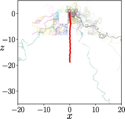
ZHENG, TOENJES, AND PIKOVSKY                                                                      PHYSICAL REVIEW E 104, 014216 (2021)

                                                                              FIG. 2. Solutions (Kl , l ) of dispersion relation (28) in (a) and
                                                                          (b) as a function of the rotation axes mean field amplitude ω̂z
                                                                          (von Mises–Fisher distribution). Panel (c) shows the roots of the
    FIG. 1. Amplitudes of the stationary mean velocity for particles      dispersion relation on the (K, ) plane for ω̂z  = 0.25. The color
with uniformly distributed rotation axes, Lorentzian frequency distri-    shade on the two branches in (a) denotes the frequency l of the cor-
bution with mean frequency ω0 = 0 (left and right handed rotations)       responding unstable mode. We see one branch having frequency zero
and width γ as a function of the noise strength D (both in units of the   (black dots), corresponding to a stationary directed mean velocity,
coupling strength). The dashed vertical lines mark the critical noise     and another branch of oscillatory instabilities (thin black line and col-
strengths according to our linear stability analysis of the incoherent    ored circles). Depending on K one of these two types of instabilities
state, Eqs. (31) and (32). The solid red line on top of the simulations   occurs first when ω̂z  increases. The dashed horizontal line marks
for γ /K = 0 is the mean field amplitude (9) for the globally coupled     the coupling K = 1.38 in the examples of Fig. 3. The dashed vertical
Vicsek model (von Mises–Fisher distribution).                             lines mark the values ω̂z  = 0.08, 0.2 and 0.38 corresponding to
                                                                          the horizontal lines in Fig. 3(a). The first instability at ω̂z  = 0.08
it to be the sum of three components: (i) a constant rotation             corresponds to a directed motion; the second, oscillatory unstable
bias of amplitude ωi around a rotation axis in the direction              mode appears at ω̂z  = 0.31. This can be seen in the magnified
ω̂i ; (ii) an alignment force which rotates σ̂ i towards a vector         plot in (b). At ω̂z  = 0.25 we show in panel (c) critical coupling
ρi (this component is responsible for interaction of the units);          values for the unstable modes and corresponding frequencies (dark
                                                                          green circles). At these points the real part (light red lines) and the
and (iii) a noise component ξ i :
                                                                          imaginary part (black lines) of the dispersion relation Eq. (28) vanish
                μi = ωi ω̂i + K (σ̂ i × ρi ) + ξ i (t ).           (2)    simultaneously. The three oscillatory modes are part of the same
                                                                          (colored) branch in panel (a).
Here K is a coupling strength which, when it is positive,
promotes alignment of σ̂ i with ρi . The term ξ i (t ) is a vector
of independent Gaussian white noises (ξ i )n (t )(ξ j )m (t  ) =       is taken to be larger than the spatial size of the     popula-
2Dδi j δmn δ(t − t  ). The Langevin equation (1) with stochastic         tion, the coupling becomes global, i.e., ρi = ρ = N1 i σ̂ i =
force (2) is to be interpreted in the sense of Stratonovich               σ̂. Below we consider globally coupled populations only.
to preserve the unit amplitude of the vectors σ̂ i . By direct            The amplitude ρ = |ρ| serves as the order parameter for the
simulation of the model we observe that a positive global                 synchronization/alignment transition. It takes values between
coupling above some critical value leads to an alignment                  zero for a uniform distribution of σ̂ i and one when the vectors
(synchronization) of the units, as shown in Figs. 1 and 3. The            are identical.
goal of the analysis below is to understand this transition.                  In the thermodynamic limit N → ∞ the system can be
                                                                          described by a family of smooth densities f (σ̂, t; ω̂, ω) for
                                                                          vectors σ̂ with a given fixed rotation bias ωω̂. These densities
                    B. Fokker-Planck equation
                                                                          obey the Fokker-Planck equation
   In the standard Vicsek model [5] with local interactions,
the variables σ̂ i are particle velocities v̂ i , the constant rotation                       ∂t f + ∇ s · ( f a) = D∇ 2s f ,                  (3)
bias is zero (ωi ω̂i = 0) and the vector ρi is the average velocity
of all particles within a distance R from the ith particle. As a          where ∇ s is the vector differential operator along the surface
result of the competition between the aligning coupling and               of a unit sphere acting on the argument σ̂ and a = ωω̂ × σ̂ +
noise, there exists a critical coupling strength Kcr , at which the       K (ρ − (ρ · σ̂)σ̂ ) is the deterministic part of the force acting on
incoherent state loses stability. When the radius of interaction          a vector σ̂ with rotation bias ωω̂.

                                                                    014216-2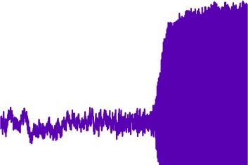
TRANSITION TO SYNCHRONY IN A … PHYSICAL REVIEW E 104, 014216 (2021)
value
∞
ρ= dω g(ω) r(ω̂, ω)G(ω̂) dA(ω̂) (4)
−∞ S2
of the frequency dependent mean fields
r(ω̂, ω) = σ̂ f (σ̂, t; ω̂, ω) dA(σ̂ ). (5)
S2
The terms dA denote the S 2 surface volume elements.
III. DIFFUSION ON A SPHERE WITH GLOBAL COUPLING
A. Synchronization and alignment transition
The simplest case allowing for a full analytic treatment is
the one without oscillations, i.e., g(ω) = δ(ω). Then the two
processes determining the dynamics of vectors σ̂ are diffusion
under the influence noise and alignment to the mean field ρ:
σ̂˙i = [K (σ̂ i × ρ) + ξ] × σ̂ i . (6)
The stationary solution of the Fokker-Planck equation (3) can
be found analytically. It is current ree, which amounts to a
detailed balance condition in (3):
f a = f · K (ρ − (ρ · σ̂ )σ̂) = D∇ s f . (7)
Without loss of generality, we set ρ = ρẑ and multiply both
sides of Eq. (7) by ẑ. The resulting one-dimensional differ-
ential equation for the rotational symmetric density has the
Boltzmann-type von Mises–Fisher distribution as a solution:
Kρ Kρ
f (θ , φ) = f (θ ) = Kρ exp cos θ . (8)
4π D sinh D D
Here θ , φ are polar angles defining the direction of the vector
σ̂. For this density Eqs. (4) and (5) give the self-consistency
condition
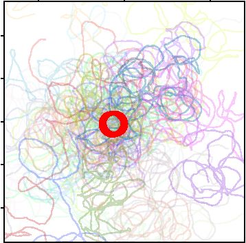
FIG. 3. Transient and final states of N = 10 000 particle veloci- Kρ D
|ρ| = ρ = coth − . (9)
ties and frequency vectors with K = 1.38, noise level D = 0.2, mean D Kρ
rotation frequency ω0 = 1.0, and frequency heterogeneity γ = 0.05.
Its solution can be represented in a parametric form. Denoting
The directions of the rotation axes evolve from uniformly random
initial conditions under the influence of mean field coupling κ and
x = KρD
, we obtain both the order parameter ρ and the essen-
angular diffusion d = 0.005. In the left column κ = 0.0158 and in tial parameter of coupling to noise ratio K/D as functions of
the right column κ = 0.018. Panels from top to bottom show (a) the x: ρ = coth x − 1/x and K/D = x 2 /(x coth x − 1). The auxil-
mean field amplitude ω̂z of the rotation axes (rising, dark blue iary parameter 0 < x < ∞ varies between the transition point
curves) and the deviation from the von Mises–Fisher distribution at x → 0, where ρ → 0, and the noise-free limit x → ∞,
[Eq. (15), flat, light curves] as functions of time; (b) the final station- where ρ → 1 (complete alignment). These analytic expres-
ary distribution of rotation axes directions as small dots on the unit sions are in agreement with direct simulations of Eq. (6), as
sphere (sinusoidal projection) and a large circle in the direction of depicted in Fig. 1 (case γ /K = 0). Expanding Eq. (9) to the
the mean field ω̂; (c) the velocity mean fields ρz (light red curve, in third order in ρ we obtain close to the transition point
the direction of ω̂) and ρx (dark purple curve) as functions of time;
(d) the final stationary or rotating distribution of particle velocities Kρ K 3ρ3 15D2 (K − 3D)
ρ≈ − 3
or ρ ≈ , (10)
(small dots) and the direction of the velocity mean field (large circle); 3D 45D K3
and (e) sample particle trajectories in the final state over t = 100 time i.e., the globally coupled Vicsek model has a continuous tran-
units (thin irregular lines) as well as the full ensemble center of mass sition at K = 3D with critical exponent 1/2.
trajectory (bold line). Horizontal and vertical dashed lines in panels
(a) and (c) are discussed in the text.
B. A model for von Mises–Fisher distribution of rotation axes
In this paper we assume that the frequencies ω and Above in Sec. III A we considered a simple situation with-
the rotation axes ω̂ are random and independent. They are out rotation biases. Below we perform a more general analysis
distributed according to the probability densities g(ω) and that includes distributions of the frequencies g(ω) and of the
G(ω̂), respectively. The order parameter ρ is the expectation rotation axes G(ω̂). The latter is a distribution on a sphere,
014216-3ZHENG, TOENJES, AND PIKOVSKY PHYSICAL REVIEW E 104, 014216 (2021)
and it is natural to assume it belongs to the von Mises–Fisher In order to solve Eq. (17), we express σ̂ and η(θ , φ, ω) in
family of distributions (because this family spans a range from terms of bi-orthonormal spherical harmonics Ylm (θ , φ) as
the uniform to a very narrow distribution). As it follows from ⎛ −1 ⎞
the analysis above, a von Mises–Fisher distribution naturally Y − Y11
2π ⎝ 1−1
appears as a stationary distribution for the Langevin process σ̂ = iY1√ + iY11 ⎠ (18)
3
(6). Therefore, below we use the model where rotation axes 2Y10
ω̂i are not constants, but evolve slowly like in (6):
and as
ω̂˙i = [κ (ω̂i × ω̂) + ζ] × ω̂i . (11) ∞
l
η(θ , φ, ω) = bml (ω)Ylm . (19)
where ζ with (ζ i )n (t )(ζ j )m (t ) = 2dδi j δmn δ(t − t ) is Gaus- l=0 m=−l
sian white noise. If the coupling κ and the noise intensity d are
small, the evolution of the distribution G(ω̂, t ) according to On the surface of the sphere the action of the diffusion term re-
(11) is slow. Furthermore, as will be illustrated below, during duces to ∇ 2s Ylm (θ , φ) = −l (l + 1)Ylm (θ , φ). Substituting this
this evolution G(ω̂, t ) is a slowly evolving von Mises–Fisher expansion into Eq. (17), we obtain a linear system of equa-
distribution. This is confirmed in Fig. 3 below by monitoring tions for the coefficients bml :
the ensemble moments ω̂z , ω̂z2 , ω̂x2 , and ω̂y2 . According 1 √
to (9) for a von Mises–Fisher distribution (8) of rotation axes √ K 2ρzY10 + (ρx + iρy )Y1−1 − (ρx − iρy )Y11
6π
κω̂z κω̂z ∞
l
fω (θ , φ) = κω̂z exp cos θ , (12)
4π d sinh d d = bml [s + imω + Dl (l + 1)]Ylm (θ , φ), (20)
l=0 m=−l
which for d < 3κ has the second moments
which can be solved using the orthonormality of the spherical
harmonics. Since the left-hand side depends on Ylm with l = 1
ω̂z2 = 1 − 2d/κ, (13)
only, the components bml with l > 1 decay exponentially at
rates Dl (l + 1). For l = 1 the coefficients b01 , b−1 1
1 , and b1 are
ω̂x2 = ω̂y2 = d/κ, (14)
calculated explicitly, resulting in the general form
the deviation
1 Kρz 0 1 K (ρx + iρy ) −1
η(θ , φ, ω) = Y + Y
ω̂x2 ω̂z 3π s + 2D 1 6π s + 2D − iω 1
= ω̂z + − coth (15)
ω̂z ω̂x2 1 K (ρx − iρy ) 1
− Y (21)
6π s + 2D + iω 1
must be zero. We check numerically, that in our simulations
this is not only valid in the final stationary state, but also of a potentially unstable mode. Integrating σ̂η over the sur-
during the transient. This allows us to study the synchroniza- face of the sphere [Eqs. (5), (18), and (21)], using again
tion transition in an adiabatically evolving von Mises–Fisher the orthonormality of the spherical harmonics, we obtain the
distribution of the rotation axes. frequency dependent mean fields (moments of the linear per-
turbation) to linear order:
⎛ ρx λ−ρy ω ⎞
IV. LINEAR STABILITY ANALYSIS OF THE
λ2 +ω2
INCOHERENT STATE 2K ⎜
⎜
⎟
ρy λ+ρx ω ⎟
r= σ̂η(θ , φ, ω)dA(σ̂ ) = ⎝ 2 +ω2 ⎠
, (22)
3 λ
In the following we analyze the stability of the incoherent S1
ρz
state where the vectors σ̂ (or velocities v̂) are distributed λ
,
uniformly in all directions and |ρ| = ρ = 0. Following the where λ = s + 2D. According to the convention above, ω̂ is
nontrivial derivation in [10], the Fokker-Planck equation (3) directed along ẑ while the direction of ρ is arbitrary. However,
can be rewritten as expression (22) can be rewritten in a covariant form, allowing
∂f for arbitrary directions of ρ and ω̂:
+ K (∇ s f − 2 f σ̂) · ρ + (ωω̂ × σ̂ ) · ∇ s f = D∇ 2s f . (16)
∂t 2K λρ ωω̂ × ρ 1 λ
r= + + − ω̂( ω̂ · ρ) .
We consider a small perturbation on top of the uniform inco- 3 λ2 + ω 2 λ2 + ω 2 λ λ2 + ω 2
herent distribution f0 = (4π )−1 . Substituting the ansatz f = (23)
f0 + η(σ̂, ω̂, ω)est for a small perturbation into Eq. (16) and To express the resulting dispersion relation equation, it is
assuming without loss of generality ω̂ = ẑ (this allows us to convenient to introduce the following notations:
express the eigenmode in terms of angles θ , φ), we obtain to (1) We introduce the averages over the distribution of the
the linear order in ρ and η the equation frequencies as
∞ ∞
λ ω
∂ h1 = g(ω)dω, h = g(ω)dω,
2K (ρ · σ̂)(4π )−1 = ω η(θ , φ, ω) −∞ λ + ω
2 2 2
−∞ λ + ω
2 2
∂φ
(24)
+ sη(θ , φ, ω) − D∇ 2s η(θ , φ, ω). (17) and h3 = λ1 − h1 .
014216-4TRANSITION TO SYNCHRONY IN A … PHYSICAL REVIEW E 104, 014216 (2021)
(2) We introduce two matrices, characterizing the distribu- Kuramoto model [10]. Indeed, in two dimensions the connec-
tion of the rotation axes: the antisymmetric matrix of the first tion between the Vicsek model and the Kuramoto model has
moments as been made explicit [17,18]. The three-dimensional Kuramoto
⎛ ⎞ model without noise was discussed as a swarming model
0 −ω̂z ω̂y
⎝ ω̂z in [10]. Strikingly and in stark contrast to the classical Ku-
= 0 −ω̂x ⎠G(ω̂)dA(ω̂) (25)
ramoto model, despite heterogeneous frequency amplitudes
S1 −ω̂y ω̂x 0
and rotation directions, which were described in [10] as im-
and the covariance matrix W as perfections that make individuals deviate from ideally straight
⎛ 2 ⎞ lines, global coupling leads to a finite translational collective
ω̂x ω̂x ω̂y ω̂x ω̂z motion for arbitrary small coupling strength, when all oscilla-
W= ⎝ω̂x ω̂y ω̂y2 ω̂y ω̂z ⎠G(ω̂)dA(ω̂). (26) tions cease as the velocities settle at well-defined fixed points.
ω̂x ω̂z ω̂y ω̂z ω̂z2
S 1
Frequency heterogeneity is not sufficient to prevent velocity
alignment.
With these notations we can express ρ from (4) and (23)
On the other hand, random perturbations of the torque in
self-consistently in a compact form
the form of Gaussian white noise stabilize the incoherent state,
2K much as in the classical Kuramoto model, and a transition
ρ= [h1 1 + h2 + h3 W]ρ. (27) to collective motion occurs at finite coupling strength. In
3
Fig. 1 we show the mean velocity as a function of the relative
The real part of the exponent s = λ − 2D for any mode ρ noise strength D/K for an isotropic distribution of rotation
matching this eigenvalue equation gives the growth rate of axes G(ω̂) = 1/(4π ) and Lorentzian frequency distributions
that mode. Equation (27) has a nontrivial solution ρ if the g(ω) = πγ (ω2 + γ 2 )−1 with mean frequency zero and width
dispersion relation γ characterizing the frequency heterogeneity. Depending on
the ratio γ /K a stationary mean field bifurcates continuously
2K
det (h1 1 + h2 + h3 W) − 1 = 0 (28) from ρ = 0 at a critical value of (D/K )cr , which the linear
3
stability analysis in Sec. VI A predicts.
holds. This is the main result of our paper and we will discuss The branch of partially synchronized states stretches from
consequences and examples in the following sections. But this bifurcation point on the horizontal axis (where ρ = 0) to
first we would like to examine general properties of Eq. (28). a point on the vertical axis (at D = 0) in the noise free limit,
Because both the real and the imaginary part of the deter- discussed in [10]. The existence of a critical ratio (D/K )cr
minant (28) must be zero at criticality where s = i and for the transition from incoherence to coherence means that
other system parameters are fixed, this occurs at a discrete the noise free limit D → 0 is singular as the critical coupling
set of points (Kl , l ) (see an example in Fig. 2 below). At strength also goes to zero. In Fig. 1 we show four examples
the smallest coupling strength Kcr = minl Kl , the incoherent with different frequency heterogeneities γ /K = 0, 0.1, 1, and
state loses stability and a nonzero mean field with frequency 10. The rotation-free case γ /K = 0 corresponds to the glob-
cr emerges. For any critical mode with (Kl , l ) the mode ally coupled Vicsek model for which the bifurcation curve
with (Kl , −l ) is also critical. Moreover, there is always at is known parametrically [Eq. (9), solid red line]. When the
least one nonoscillating solution (Kl , l = 0) since the deter- frequencies are very heterogeneous, e.g., γ /K = 10, the in-
minant is a cubic polynomial in K with real coefficients when coherent state, where the mean velocity is zero, is stable for
= 0. A nonzero frequency cr at the bifurcation indicates even lower ratios of D/K. For D = 0 the mean velocity in the
the formation of a rotating velocity mean field in the swarming limit γ /K → ∞ is ρ = 0.5 corresponding to the limit K → 0
model where the variables are interpreted as velocities σ̂ = v̂. as predicted in [10].
This means that the population will demonstrate coherent
oscillations. In contradistinction, if the critical mode has zero VI. AXIAL-SYMMETRIC DISTRIBUTION OF
frequency cr = 0, a transition to a regime with a stationary ROTATING AXES
nonzero mean velocity occurs. This corresponds to a directed
motion of the swarm’s center of mass. In this section we go beyond the simplest setup of Sec. V
The dependence of the real and imaginary parts of the and discuss a nontrivial situation where there is a preferable
matrix determinant in (28) on the system parameters can be direction of rotation axes ω̂.
arbitrary complicated [see Fig. 2(c)]. Changing the system pa-
rameters, pairs of points (Kl , l ) can emerge or annihilate and A. The general case
the sequence of critical coupling strengths for these unstable
With ẑ-axial symmetry of the distribution G(ω̂), the matrix
modes, and thus the type of the emerging collective motion
W (26) is diagonal and matrix (25) has only the nonvan-
can change.
ishing entries ±ω̂z . Then the matrix determinant (28) is a
product of two factors so that one of the two equations
V. SYNCHRONIZATION IN THE PRESENCE OF A
3
UNIFORMLY DISTRIBUTED ROTATION BIAS 0 = h1 + ω̂z2 h3 − , (29)
2K
In the presence of individual, quasistatic rotation axes, the 2
3
model described by Eqs. (1) and (2) is a noisy version of 0 = h1 + ω̂x2 h3 − + ω̂z 2 h22 (30)
the recently proposed three-dimensional generalization of the 2K
014216-5ZHENG, TOENJES, AND PIKOVSKY PHYSICAL REVIEW E 104, 014216 (2021)
must hold. If ω̂z h2 is zero, one can show that no oscillatory distribution completely and we can study the linear stability
instabilities with = 0 exist. This includes also the cases as a function of ω̂z alone.
discussed in Sec. V. Then the numbers of left and right ro- We start with a discussion of linear stability properties
tating oscillators around each rotation axis are equal and we of the uniform incoherent state, according to the analytical
can immediately find the solutions with = 0 as expressions of Sec. IV. Figures 2(a) and 2(b) shows the crit-
ical coupling strength and frequency of unstable modes as a
3 1
K= , (31) function of ω̂z according to our linear stability analysis [the
2 ω̂2 h3 + h1 λ=2D roots of Eq. (28) are found numerically]. There are two critical
where ω̂2 = ω̂z2 for Eq. (29) and ω̂2 = ω̂x2 = ω̂y2 for branches. One (black) branch corresponds to a transition to a
Eq. (30). The smaller of these two K values is the critical non-oscillating mode, and thus to a directed motion of parti-
coupling strength. With a Lorentzian frequency distribution cles. Another (colored) branch corresponds to an oscillating
g(ω) = π1 (ω−ωγ0 )2 +γ 2 , the integrals (24) and h3 = 1/λ − h1 can mode, and thus to center-of-mass oscillations in the popula-
directly be calculated: tion. We choose the coupling parameter K = 1.38, therefore
with a gradual increase of ω̂z the system evolves along a
λ+γ ω0 horizontal line in Figs. 2(a) and 2(b). The first transition at this
h1 = , h2 = . (32)
(λ + γ )2 + ω02 (λ + γ )2 + ω02 coupling strength is to a nonoscillating mode at ω̂z ≈ 0.08.
At ω̂z ≈ 0.32 an oscillating mode also becomes unstable.
Inserting these expressions into (30) and (29) gives an explicit
From the linear analysis we cannot judge, what will be a result
formula for the critical coupling strength. To calculate the
of a competition of these modes.
critical coupling strength in Fig. 1, where ω0 = 0 and ω̂2 =
Figure 3 shows results of direct numerical simulations,
1/3, we use Eq. (31). Equation (31) with a delta distribution
with the aim to test the prediction of the linear stability
of frequencies, i.e. ω = ω0 and γ = 0, gives the exact same
analysis and to explore truly nonlinear regimes. We have
result as in Ref. [15] which is thus included in our analysis as
chosen two values of rotation axes coupling, κ = 0.0158 in
a special case.
the left column and κ = 0.018 in the right column of Fig. 3.
The difference is that for the former, smaller value of κ the
B. Example: Slowly evolving von Mises–Fisher distribution saturation level of ω̂z does not exceed the critical value for
When chiral symmetry is broken, i.e., ω̂z h2 = 0, oscilla- the oscillatory instability. Thus, here we expect the directed
tory instabilities can be expected, leading to a partial phase motion to occur. This is indeed observed in the simulations.
synchrony of the helical trajectories. In this case the swarm The directed motion itself is illustrated in panel (e1), where
center of mass can perform quite regular oscillations whereas one can see that it is superimposed with helical trajectories
individual trajectories appear to be erratic [see Fig. 3(e2)]. of the particles. The transition point is, however, delayed
Such collective oscillations have recently been observed in in comparison to the theoretical prediction: it happens at
dense colonies of E. coli [7]. time t ≈ 4000 [see panel (c1)], where the value of ω̂z is
As an example shown in Figs. 2 and 3, we study the 0.2. A delay of bifurcation (compared to the static value
transition to collective motion in a swarm of globally coupled, ω̂z = 0.08) is a general phenomenon for parameter-varying
self propelled particles of unit velocities v̂ and with helical systems; here it might be even enhanced due to finite-size
trajectories. The rotation axes ω̂ of the particles diffuse and effects.
align slowly to their mean direction according to Eq. (11) Another, larger value of κ = 0.018 leads to a saturated
with d = 0.005 and κ = 0.0158 or κ = 0.018. We use these level of the alignment of rotation axes at ω̂z ≈ 0.5, which
two values to illustrate directed and rotating motions of the is larger than the second critical value for the instability of the
particles center of mass. The frequency distribution g(ω) is oscillating mode. Here we observe two transitions, as one can
Lorentzian with mean frequency ω0 = 1.0 and width γ = see in panel (c2) of Fig. 3. The first transition at t ≈ 1500 cor-
0.05. The coupling strength and the diffusion constant for the responds to the same value ω̂z ≈ 0.2 as in panel (c1). In this
velocity vectors are K = 1.38 and D = 0.2. transition a directed motion with ρz = 0 appears. However,
We can apply our linear stability analysis under the as- this motion is a transient episode: it exists only up to time
sumption of a quasistatic distribution of rotation axes ω̂. We t ≈ 2000, at which the alignment of frequencies reaches level
start with isotropic random initial conditions of uniformly dis- ω̂z ≈ 0.38. Starting from this level, the oscillating mode
tributed axes ω̂, where the incoherent distribution of velocities dominates: a rotation of ρ in the x-y plane with ρz ≈ 0 and
σ̂ is stable for K = 1.38. As the rotation axes evolve accord- oscillating values of ρx and ρy [panel (c2)]. The rotational
ing to (11), they start to align and ω̂z grows, the moment motion of the center of mass is illustrated in panel (e2).
ωz2 is growing, and the moments ωx2 = ωy2 = 1 − 2ωz2
are decreasing. With these parameters, the linear stability of
VII. CONCLUSION
the incoherent velocity distribution changes as well. At some
point it can become linearly unstable, the velocity vectors start In conclusion, we have investigated velocity alignment and
to align, and a transition to collective motion is observed. frequency synchronization in a three-dimensional globally
During the transient we monitor deviation of the rotation coupled swarming model with helical trajectories and noise.
axes distribution from the von Mises–Fisher distribution ac- Unit velocity vectors of the particles precess around individual
cording to Eq. (15). One can see in Fig. 3(a) that systematic rotation axes, tend to align into the direction of the mean
deviations are smaller than finite ensmble size fluctuations in velocity due to coupling, and are subject to noise. We have
the equilibrium state, i.e., ω̂z characterizes the rotation axes derived the condition for the emergence of a nonzero velocity
014216-6TRANSITION TO SYNCHRONY IN A … PHYSICAL REVIEW E 104, 014216 (2021)
mean field, leading to either a directed motion of the swarm type and the characteristic exponents of the synchronization
or to collective oscillations. In direct simulations we have only transition.
observed second-order transitions at finite coupling strength,
in contrast to a discontinuous transition at infinitesimal small
ACKNOWLEDGMENTS
coupling, reported in the singular, deterministic limit [10].
A higher order analysis beyond linear stability considera- C.Z. acknowledges financial support from the China Schol-
tion, such as the multiscale perturbation method used in the arship Council (CSC). A.P. was supported by the Russian
classical Kuramoto model, is still needed to characterize the Science Foundation, Grant No. 17-12-01534.
[1] E. Lauga and T. R. Powers, Rep. Prog. Phys. 72, 096601 [9] H. Chaté, F. Ginelli, G. Grégoire, and F. Raynaud, Phys. Rev. E
(2009). 77, 046113 (2008).
[2] C. Bechinger, R. Di Leonardo, H. Löwen, C. Reichhardt, G. [10] S. Chandra, M. Girvan, and E. Ott, Phys. Rev. X 9, 011002
Volpe, and G. Volpe, Rev. Mod. Phys. 88, 045006 (2016). (2019).
[3] S. Tottori, L. Zhang, F. Qiu, K. K. Krawczyk, A. Franco- [11] S. Watanabe and S. H. Strogatz, Physica D 74, 197 (1994).
Obregón, and B. J. Nelson, Adv. Mater. 24, 811 (2012). [12] E. Ott and T. M. Antonsen, Chaos 18, 037113 (2008).
[4] H. Xie, M. Sun, X. Fan, Z. Lin, W. Chen, L. Wang, L. Dong, [13] T. Tanaka, New J. Phys. 16, 023016 (2014).
and Q. He, Sci. Rob. 4, eaav8006 (2019). [14] S. Chandra, M. Girvan, and E. Ott, Chaos 29, 053107 (2019).
[5] T. Vicsek, A. Czirók, E. Ben-Jacob, I. Cohen, and O. Shochet, [15] F. Ritort, Phys. Rev. Lett. 80, 6 (1998).
Phys. Rev. Lett. 75, 1226 (1995). [16] T. Niedermayer, B. Eckhardt, and P. Lenz, Chaos 18, 037128
[6] A. Attanasi et al., Phys. Rev. Lett. 113, 238102 (2014). (2008).
[7] C. Chen, S. Liu, X.-q. Shi, H. Chaté, and Y. Wu, Nature [17] A. Chepizhko and V. Kulinskii, Physica A 389, 5347 (2010).
(London) 542, 210 (2017). [18] P. Degond, G. Dimarco, and T. B. N. Mac, Math. Models
[8] G. Grégoire and H. Chaté, Phys. Rev. Lett. 92, 025702 (2004). Methods Appl. Sci. 24, 277 (2014).
014216-7You can also read