Supplement of The influence of layering and barometric pumping on firn air transport in a 2-D model

Supplement of The Cryosphere, 12, 2021–2037, 2018
https://doi.org/10.5194/tc-12-2021-2018-supplement
© Author(s) 2018. This work is distributed under
the Creative Commons Attribution 4.0 License.

Supplement of
The influence of layering and barometric pumping on firn air
transport in a 2-D model
B. Birner et al.

Correspondence to: Benjamin Birner (bbirner@ucsd.edu)

The copyright of individual parts of the supplement might differ from the CC BY 4.0 License.

1 2D trace gas transport model

 1.1 Numerical integration scheme

10 Trace gas migration in firn is governed by the following partial differential equation (Eq. (2) in main text)

 ̃ = ∇ ⋅ [ ̃ (∇ − + Ω ̂ )] + ∇ ⋅ [ ̃ ∇ ] − ( ̃ ) ⋅ ∇ ,
 (S1)
 
 ∆ M 
 where ≡ , ≡ + 1 is the trace gas or isotope mixing ratio, ̃ ≡ exp ( ) pressure-corrected open porosity
 1000 

 (m3 m-3), temperature (K), ∆ isotope mass difference (kg mol-1) to the mass of air M (kg mol-1), gravitational acceleration
 (m s-2), the fundamental gas constant (J mol-1 K-1), air advection velocity due to snow accumulation, pore compression
 and barometric pumping (m s-1), and Ω thermal diffusion sensitivity (K-1). is the molecular diffusivity and is the
15 dispersion tensor (m2 s-1). has different entries on the diagonal to represent different strengths of molecular diffusion in
 the vertical and horizontal direction. Similarly, is simplified to an “eddy diffusivity”, , acting in vertical and horizontal
 direction as described in the text. ̃ = ̃ ( ), = T(z, t), and = ( , , ) are scalar fields. Furthermore, = ( , , ) ̂ +
 
 ̂ is a vector field and ∇ ≡
 ( , , ) ̂ + ̂ is the gradient operator in 2D.
 
 Equation (S1) is discretized using a Crank-Nicolson time stepping scheme and central difference approximations derived
20 from flux balance on an Arakawa C (i.e., staggered; Fig. S1) grid as follows:

 ( , , + ∆ ) − ( , , ) 1
 ̃ ( ) = [( + )| +∆ ( , , + ∆ ) + ( + )| ( , , )] , (S2)
 ∆ 2

 where

 1

∆ ∆ ∆ 
 − ̃ ( + , , ) ̃ ( − , , ) ̃ ( , + , )
 2 2 2
 | ( , , ) ≡ ( + ∆ , , ) + ( − ∆ , , ) − ( , + ∆ , ) +
 2∆ 2∆ 2∆ (S3)
 ∆ ∆ ∆ ∆ ∆ 
 ̃ ( , − , ) ̃ ( + , , ) − ̃ ( − , , ) ̃ ( , + , ) − ̃ ( , − , )
 2 2 2 2 2
 ( , − ∆ , ) + [ + ] ( , , ) ,
 2∆ 2∆ 2∆ 

 ∆ ∆ ∆ ∆ 
 ̃ ℎ∗ ( + , , ) ̃ ℎ∗ ( − , , ) ̃ ∗ ( , + , ) ̃ , ( , + , )
 2 2 2 2
 | ( , , ) ≡ ( + ∆ , , ) + ( − ∆ , , ) + [ − +
 ∆ 2 ∆ 2 ∆ 2 2∆ 

 ∆ ( , +∆ , )− ( , , ) ∆ ∆ 
 ̃ , Ω( , + )( ) ̃ ∗ ( , − , ) ̃ , ( , − , )
 2 ∆ 2 2
 ] ( , + ∆ , ) + [ + −
 2∆ ∆ 2 2∆ 

 ∆ ( , , )− ( , −∆ , ) ∆ ∆ ∆ ∆ 
 (S4)
 ̃ , Ω( , − )( ) ̃ ℎ∗ ( + , , )+ ̃ ℎ∗ ( − , , ) ̃ ∗ ( , + , ) + ̃ ∗ ( , − , )
 2 ∆ 2 2 2 2
 ] ( , − ∆ , ) + [− 2 − 2 +
 2∆ ∆ ∆ 

 ∆ ∆ ∆ ( , +∆ , )− ( , , ) ∆ ( , , )− ( , −∆ , )
 ̃ , ( , − , ) − ̃ , ( , + , ) ̃ , Ω( , + )( )− ̃ , Ω( , − )( )
 2 2 2 ∆ 2 ∆ 
 + ] ( , , ) ,
 2∆ 2∆ 

 with ∗ ≡ + a combination of eddy and molecular diffusivity in vertical ( ∗ ) and horizontal ( ℎ∗ ) direction, ∆ time
 step of integration (s), ∆ vertical grid spacing (m), and ∆ horizontal grid spacing (m). Here ̃ , , , Ω, ℎ∗ , ∗ , , and are
 Nx1 vector where N is the number of grid cells; and are banded square-matrices of dimensions NxN that represent the
 advection operator (i.e., the sum of the three velocity components) and the diffusion operator (Fickian diffusion, eddy diffusion,
 5 thermal diffusion, and gravitational fractionation), respectively. The two matrices have entries on the diagonal as well as four
 off-diagonals corresponding to the grid points above, below, to the left and to the right. Because and are also dependent
 on time, subscripts indicate the time step in Eqs. (S3) and (S4). Equations (S2) – (S4) form a system of linear equations
 describing the change in time of at all spatial points. Rearranging Eq. (S2) yields

 −1 ∆t
 ( , , + ∆ ) = [ ̃ ( ) − ( + )| +∆t ] [ ( + )| + ̃ ( ) ] ( , , ) , (S5)
 2

 with the identity matrix, which can be stepped forward in time. In the limit of no horizontal transport and constant coefficients
10 ( ̃ , , and constant), we find good agreement between this numerical model and analytical solutions for a simple 1D
 model (Appendix A, Fig. S2). δ15N profiles from the model run at 5x higher temporal resolution indicate that the error
 introduced by a coarser time step converges and is small (~0.5 per meg) relative to the signal in the deep firn (~5 per meg)
 (Fig. S3).

 2

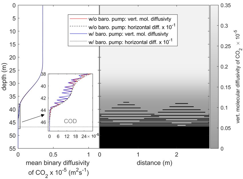
Figure S1. Schematic of how variables , , , ̃ , D*, Ω and are defined on the staggered grid.

 Figure S2. Comparison of 1D analytical solutions (Appendix A, solid lines) and numerical model output (dashed coloured lines). Here =
5 10−9 m s-1, = 6 × 10−7 m2 s-1 and molecular diffusivity of CO2 = 6 × 10−6 m2 s-1 up to the COD. The dashed black line shows the
 gravitational settling equilibrium, i.e., the steady-state solution for each isotope pair neglecting advection and non-fractionating mixing
 processes ( ).

 3

Figure S3. Evolution of the root-mean-square difference between the δ15N profile produced by the model with barometric pumping and a
 time step of 3.5 days (default setting) relative to results obtained with 5x higher temporal resolution (assumed to yield the “true” solution).
 The error is quantified in the depth range of 68-75 m at WAIS Divide and converges at less than 0.1 per meg after ~15 years. The pressure
 5 forcing was linearly interpolated for the high-resolution run and the model was initialized with the steady-state solution presented in the
 main text for both time steps. Interannual variability in the plot is caused by different surface pressures conditions right before each data
 point was recorded which forced transport of more or less gravitationally fractionated air into the region of interest.

 1.2 Layering

 We solve the trace gas transport equation under the consideration of discontinuous, impermeable, horizontal layers. Owing to
10 computational limitations, layers are somewhat idealized by assigning them an infinitesimal thickness.
 Layers are advected with the firn. The z-axis position of layer , at time t, is found by numerically integrating the equation
 
 ( ) = ( 0 ) + ∫ ( ( ′ )) dt′ , (S6)
 0

 from the initial time 0 where is the depth of the layer and is the vertical firn advection velocity. Equation (S6) is
 discretized using Forward Euler time stepping such that

 ( ) = ( − ∆t) + wfirn (zl (z − ∆t))∆t . (S7)

 Layer positions on the discrete grid are updated once a layer has moved below the depth of the next grid box. New layers
15 are introduced at 70% of the total depth of the firn column once the top layer was displaced by at least the thickness of one
 annual layer from its initial position. The centre of each layer opening alternates between two locations (separated by half the
 horizontal domain length) and the layer size increases linearly with depth. Layers begin to cover the entire horizontal range of
 the model when the COD is reached and are not tracked further below this depth because any further gas transport is limited
 to advection with the pores.

20 1.3 Boundary conditions

 A set of boundary and initial conditions accompany Eq. (S1):
 4

1) The model is initialized with isotopic ratios as expected from gravitational equilibrium at all depths. For CO2 and CH4
 transport simulations, initial concentrations are set to the lowest atmospheric concentrations observed for the time window
 of the simulation.
 2) Surface values of q are given by the atmospheric trace gas concentration at each time step (i.e., a Dirichlet boundary).
 5 Atmospheric isotope ratios are assumed to be constant. Atmospheric CO2 and CH4 histories are taken and updated from
 Buizert et al. (2012) based on a combination of direct measurements and reconstructions from the Law Dome ice core site
 (Figure S4) (Etheridge et al., 1996, 1998; Keeling et al., 2001; Dlugokencky et al., 2016a, 2016b).
 3) A periodic boundary condition is implemented for all horizontal fluxes.
 4) Because Eq. (S1) only describes the trace gas evolution in open pore space, the bottom of the domain is reached where ̃
10 equals zero. A Neumann boundary condition is chosen for this boundary and the flux leaving through the bottom of the
 domain is equal to the advection of pores with the firn. Diffusion already ceases to occur at the considerably shallower
 close-off depth (COD). Because the advective flux at the bottom boundary depends on q, it must be approximated locally
 using a backward difference scheme.
 5) Layers are implemented on the staggered grid by setting the diffusivity and permeability between two adjacent boxes to
15 zero. Layers have an infinitesimally small thickness and do not change the porosity anywhere. The permeability increases
 from layer edges towards the centre of the layer openings to obtain a more realistic flow field near layer edges. Other firn
 properties, such as the diffusivity, are changed only on layer grid points because their porosity-dependence should be
 considerably weaker than for permeability. Vertical gas advection velocities on layers correspond to the local velocity of
 firn such that mixing ratio discontinuities are preserved and correctly advected downward at the same speed as layers.
20 Layers do not directly impact the horizontal diffusion, permeability or porosity.

 Figure S4. Atmospheric CO2 and CH4 histories composed from a combination of direct measurements and reconstructions from the Law
 Dome ice core site (Etheridge et al., 1996, 1998; Keeling et al., 2001; Buizert et al., 2012; Dlugokencky et al., 2016a, 2016b).

 5

2 Flow field models for firn advection and barometric pumping

 2.1 Firn pore advection and pore compression

 Advection in the Eulerian frame of the model consist of 3 distinct processes that combine to form the vector u
 ⃑ in Eq. (S1). The
 first component of advection represents the downward migration of firn and air contained in the pore spaces due to the
 5 continuous accumulation of fresh snow at the surface. This flux can easily be calculated from the snow/ice mass balance and
 the density profile of the firn. Secondly, the compression of pores in the firn squeezes air out and drives a macroscopic airflow
 from the firn back to the atmosphere. Finally, barometric pumping drives direction-reversing airflows in response to surface
 pressure anomalies. These airflows act to return firn air pressures to hydrostatic balance. Barometric pumping flows are orders
 of magnitude faster than the other fluxes (Fig. 3c) but cause no net airflow when averaged over seasonal or longer time scales.
10 Nevertheless, the fast flow speeds associated with barometric pumping may produce notable dispersive mixing in the deep firn
 as discussed in the main text (Buizert and Severinghaus, 2016).
 The return and barometric pumping flows and move through the porous firn medium and obey Darcy’s law. Darcy’s
 law (Darcy, 1856) states that the equilibrium-state volume transport through the cross-sectional area A for laminar,
 incompressible flow is given by

 = − ∇ , (S8)
 
15 where is permeability of the medium (m2), is dynamic viscosity of the fluid (Pa⋅s), and ∇ is the pressure gradient
 (Pa m-1) driving the flow. We note that the hydrostatic component of pressure ( ̃ ) is no cause of flow and can thus be removed
 in the flow field model. We therefore consider only deviatoric pressure ′ ≡ − ̃. Discharge must be divided by area A
 and the pressure-corrected open porosity ̃ to obtain the true flow speed per pore-cross sectional area used in the tracer
 advection equation because only a fraction of the total area is available for flow. This results in

 = =− ∇ ′ . (S9)
 ̃ ̃

20 The continuity equation for a compressible fluid in a porous medium can be derived from the conservation equation of air
 molecules, using the ideal gas law, which yields

 ( )
 + ∇ ⋅ ( ) = , (S10)
 
 where is air density and denotes a source or sink of mass (Buizert and Severinghaus, 2016). Assuming porosity is
 ( )
 independent of time, = 0, and the density in the firn is obtained from hydrostatic balance of an isothermal atmosphere,
 
 ≃ 0 exp ( ), the continuity equation implies that
 
 6

 ̃ ( 0 )
 ∇ ⋅ ( ̃ ) = − ≡ , (S11)
 0 

 where 0 is surface air density, is a volume source or sink of air. The depth dependency of density has been absorbed into
 the open porosity as before. Equation (S11) shows that the divergence of the porosity-scaled velocity must equal the local
 source of air and change in density.
 For the return flow of air to the atmosphere (i.e., ) the source term is the compression of pores during firn advection
 5 and density changes are neglected

 = ∇ ⋅ ( ̃ ) = ∇ ⋅ [− ∇ ′ ] , (S12)
 
 and for the barometric pumping component of flow (i.e., ) the source or sink is the local density change in response to
 surface pressure anomalies

 = ∇ ⋅ ( ̃ ) = ∇ ⋅ [− ∇ ′ ] . (S13)
 
 can be calculated as the vertical derivative of the mean vertical flow due to pore compression ⟨ ⟩ = − ,
 where is the mean effective vertical air transport velocity (m s-1), such that

 = [ ̃ ( − )] . (S14)
 
10 This is analogous to calculating pore compression in a 1D firn column (Rommelaere et al., 1997). At steady-state, mass
 conservation of air requires that the net vertical flux of air molecules is equal at all depths when integrated horizontally. Using
 the ideal gas law, the total vertical transport of air molecules n per area A is given by

 = = 1 ( ̃ + ) ≡ const., (S15)
 
 where ̃ is the ambient hydrostatic pressure in open pores, is pressure of air in bubbles, and is closed porosity (m3 m-3)
 (Rommelaere et al., 1997). Temporal changes in ̃ are small and their impact on and is neglected in Eq. (S15). At =
15 (COD), vertical airflow ceases and air is only carried further downward by the advection of pores with the firn. Therefore,
 is equal to the advection velocity at and below this depth and

 1
 = ( ̃ + ) . (S16)
 | = 

 7

For given bubble pressure , Eqs. (S15) and (S16) can be solved to find and at all depths. Rommelaere et al.
 (1997) derive an equation for the change in bubble air content based on the compression of previously existing bubbles and
 the trapping of air in new bubbles

 1 
 ( ) = ∫ ̃ ( ) , (S17)
 0 

 where ≡ + is total porosity. Typical pressure profiles are shown in Fig. S5. High near the surface results from the
 5 very small, but non-zero closed porosity values that are an artefact of the porosity parameterization at that depth. Mean in
 the top ~60 % of the firn column above the COD should thus be interpreted with caution.

 Figure S5. Normalized profiles of pressure in bubbles and of hydrostatic pressure in open pores at WAIS Divide.

 Equations (S12), (S14), (S15), and (S17) are combined to calculate the pressure fields for the return flow

 [ ̃ ( − )] = ∇ ⋅ [− ∇ ′ ] . (S18)
 
10 Subsequently, the corresponding velocity field is obtained using Eq. (S9). Plots of a representative pressure anomaly field
 and corresponding flow field are shown in Figs. S6 and S7.

 8

Figure S6. Pressure anomaly field calculated for the return flow to the atmosphere shown in Fig. S7. Layers appear as discontinuities in the
 pressure field on the model domain. The plot shows a ~1 m section of the deep firn and is presented at reduced grid resolution for clarity.

 5 Figure S7. Return flow of air to the atmosphere corresponding to Fig. S6. The plot shows a selected region of the deep firn and is presented
 at reduced grid resolution for clarity. The blackness of layers indicates the local vertical permeability of the firn.

 2.2 Barometric pumping

 The source term for barometric pumping, , is equal to the change in firn air density caused by surface pressure anomalies
 associated with passing storms (Fig. S8). Air compression or expansion demands a local convergence or divergence of flow
10 that forces air to move in or out of the firn, assuming porosity remains constant.

 9

Figure S8. One-year subsection of the surface pressure forcing driving barometric pumping at WAIS Divide. Observed daily pressure
 variability of ~7 mbar was rescaled by a factor of √∆ to account for the longer time step used in the model.

 Starting from Darcy’s law, the continuity equation and hydrostatic balance, Buizert and Severinghaus (2016) derived a
 5 partial differential equation for firn air pressure similar to Eq. (S19)

 = ∇ ⋅ [ ̅0 exp ( ) ∇ ′] . (S19)
 ̃ 

 Here, we remove the hydrostatic component of pressure through the definition of ′ and use the version of Darcy’s law given
 by Eq. (S9). Note that following Buizert and Severinghaus (2016), we linearized Eq. (S19) in the pressure anomaly by replacing
 the pressure (or equivalently the density) in the continuity equation by the annual mean hydrostatic pressure
 
 ( = ̅0 exp ( )). However, the high computational costs of running a 2D model (~2 days runtime on 10 CPUs per
 
10 simulation with ∆ = 3.5 days) prevent us from reducing the time step below ~3 days and from explicitly resolving the
 propagation of surface pressure waves into firn. Instead, we assume that the pressure changes on the LHS are approximately
 in hydrostatic balance throughout the firn, in line with results by Buizert and Severinghaus (2016):

 ̃ 0 
 ≃ = exp ( ) , (S20)
 
 where 0 = 0 ( ) is the time-varying surface pressure. Combining Eqs. (S19) and (S20) yields 

 ̃ 0
 ≡ , (S21)
 ̅0 

 and an equation to calculate a hypothetical pressure field which gives rise to the barometric pumping flow

 ̃ 0 
 = ∇ ⋅ [ ∇ ′] , (S22)
 ̅0 

 10

where ̅0 is the annual mean surface pressure. The flow field, given by Eq. (S9), may be interpreted as the flow required over
 timestep ∆t to return the column to hydrostatic balance with a new surface pressure of 0 . To represent storm activity, we
 prescribe 0 ( ) as pseudo-red noise. The surface pressure variability in the model is slightly damped compared to observations
 in order to account for non-hydrostatic changes. This yields comparable mean vertical velocities as published by Buizert and
 5 Severinghaus (2016).
 Similar to Eq. (S1), the flow field models for the return flow and barometric pumping are discretized using central
 differences on a staggered grid. Values for κ are calculated using the parametrization of Adolph and Albert (2014) and is
 assumed to be constant. Surface values of ′ are set to zero for the return flow and to 0 ( ) − ̅0 for barometric pumping. The
 grid is periodic in the x-direction and no fluxes through the bottom boundary are permitted. Layers set the permeability , and
10 thus also velocities, between grid boxes to zero. Because layers are advected with the firn, the total flow field must be
 recalculated at every time step.

 3 Thermal model

 We use the thermal model of Alley and Koci (1990) to obtain temperature fields for all time steps. The temperature evolution
 of firn and ice can be simulated in 1D because horizontal temperature gradients are negligibly small. Heat transport in firn is
15 governed by a modified version of the traditional heat equation (Cuffey and Paterson, 2010)

 2 
 = 2+ − + , (S23)
 
 where = ( , ) is temperature (°C), = ( ) firn density (kg m-3), = ( ) specific heat capacity of firn (J kg-1 °C-
 1
 ), = ( , ) heat conductivity (W m-1 °C-1), vertical advection velocity of firn/ice (m s-1), and is local heat production
 due to firn compaction and ice deformation (J s-1 m-2). This expression can be rewritten in terms of the thermal diffusivity =
 
 as (Johnsen, 1977)
 
 2 2
 = 2 + [( + ) − ] +[ + ]( ) + . (S24)
 
20 Following Alley and Koci (1990), we use the following parametrizations for , cp and :

 = (1 − ), (S25)
 
 cp = 2096 + 7.7752T , (S26)

 11

 = (1 − 0.00882( + 30)) (−1.229 × 10−14 3 + 2.1312 × 10−11 2 − 9.4 × 10−9 + 1.779 × 10−6 ) , (S27)

 where is the cumulative load of firn above (kg m-2) and H the total thickness of the ice sheet. is parameterized as

 4
 ̇ 3
 2( )
 ̇ 
 (S28)
 = + 1 ,
 3 
 7217 3
 (4.26 × 10−13 exp (− ))
 + 273.15

 where ̇ is the ice equivalent accumulation rate (m s-1) (Alley and Koci, 1990). Equation (S24) is solved by explicit (forward
 Euler) time stepping because of the non-linearity in T. Spatial derivatives are approximated by central differences. Since the
 firn air transport model just requires firn temperature for the last ~200 years, only the top 130 m of the ice sheet are simulated
 5 in the temperature model for computational efficiency. The temperature gradient at the bottom boundary is fixed to zero but
 temperature at that depth can evolve freely. Surface temperature histories for WAIS Divide and Law Dome DSS were
 previously published by Orsi et al. (2012), Van Ommen et al. (1999) and Dahl-Jensen et al. (1999) and allow us to develop a
 surface forcing for the model. For the Law Dome site DSSW20K, we combine the water oxygen isotope record translated to
 temperature following Van Ommen et al. (1999) and supplement this published, six centuries long record with the rescaled
10 mean annual temperature recorded at the nearby Casey Station for the last ~50 years (Jones and Reid, 2001). Further
 information on the isotope-to-temperature scaling and the relationship to the historic data at Casey station can be found in Van
 Ommen et al. (1999). An offset is applied to the isotope and instrumental temperatures to match the slightly different mean
 annual temperature at DSSW20K compared to DSS. The Orsi et al. (2012) best fit WAIS Divide surface temperature record
 is modified slightly to bring our model results in line with the published borehole temperature profiles (Fig. S9). A site-specific
15 mean seasonal cycle is superimposed on both long-term temperature forcings. The seasonal cycle is generated by matching a
 sine and cosine wave including several harmonics to a climatology of Automated Weather Station data at WAIS Divide and
 Law Dome (Lazzara et al., 2012). The exact details of the seasonal cycle are of limited importance for trace gas transport to
 the lock-in zone because the seasonal temperature wave becomes quickly attenuated in the firn. We do not mean to imply that
 our forcings are necessarily accurate reconstructions of local surface temperature but the forcings should yield approximately
20 correct thermal gradients in the firn using our model’s temperature module. Moreover, thermal fractionation of isotopes only
 amounts to a comparatively small influence on most isotopes ratios. Thus, an approximately correct temperature profile is
 sufficient for our purposes. Temperature fields are only used to account for isotope thermal fractionation and any temperature
 influence on firn densification is neglected.

 12

Figure S9. Observed borehole temperature and simulated temperature profile at WAIS Divide in January 2009 (Data from: Orsi et al., 2012).

 13

4 Summary tables

 Table S1. Overview of important model parameters
 Parameters WAIS Divide Law Dome DSSW20K
 Firn depth (i.e., open porosity = 0) 85 m 55 m
 Model height 80.92 m 52.74 m
 Model width 2.85 m (= 12x annual layer thickness) 2.43 m
 Horizontal grid spacing 0.03 m 0.03 m
 Vertical grid spacing 0.04 m 0.04 m
 Depth of occurrence of first layer 56.65 m (= 70 % of firn depth ) 36.94 m
 Simulation time range & time step 1800–2006 in 3.5-day timesteps 1800–1998.05 in 3.5-day timesteps
 Obs. annual mean temperature T1,2 243.15 K 253.45 K
 Ice sheet thickness H 3500 m 1200 m
 Mean surface Pressure 1,2 789 hPa 850 hPa
 Surface pressure variability (1 ) 7 hPa day-1 11.2 hPa day-1
 1,2
 Ice equiv. advection velocity 6.9714×10-9 m s-1 5.1706×10-9 m s-1
 3
 Surface mixed zone eddy diffusion 0 = 2.38 × 0 0 = 2.4 × 0
 = 2.5 m = 3.5 m
 = (− )
 range: 0 – 8 m + 2 m linear taper range: 0 – 14 m + 2 m linear taper
 1
 WAIS Divide: WAIS Divide Project Members (2016)
 2
 Law Dome: Etheridge et al. (1992)
 3
 Eq. Kawamura et al. (2013)

 Table S2. Overview of selected parameterizations in the model
 Density of ice1 = 916.5 − 0.14438 ( − 273.15) − 1.517 ⋅ 10−4 ( − 273.15)2 kg m-3
 Free air diffusivities relative to CO2 Table 4 & 5 in SI to Buizert et al. (2012) and references therein
 Dispersivity2 (assumed isotropic) ( ) = 1.26 · exp(−25.7 )
 
 Total porosity = 1 −
 
 −7.6

 Closed porosity3 = 0.37 ⋅ ( )
 831.2
 1−
 
 Firn density fit 2 −zcrit2
 = − ( − (zcrit2 )) ⋅ exp [− (b1 + 2 ⋅ b2 zcrit2 )]kg m-3
 − (zcrit2 )
 WAIS Divide Law Dome DSSW20K
 Density fit parameters4 1 = 16 1 = 19.7186
 2 = 110 2 = 37.4193
 0 = 420 0 = 511.8111
 1 = 20.0121 1 = 7.8210
 2 = −151.242 2 = −0.0476
 3 = −0.1 3 = 0.4143
 0 = 506.85 0 = 556.5176
 1 = 5.3748 1 = 5.3204
 2 = −0.0152 2 = 0.0117
5 1
 Eq: Schwander et al. (1997)
 2
 original Eq: Buizert and Severinghaus (2016)
 3
 Eq: Goujon et al. (2003) in Severinghaus et al. (2010) and Kawamura et al. (2013)
 4
 data: Trudinger et al. (1997); WAIS Divide coefficients: Battle et al. (2011)

 14

5 Law Dome DSSW20K firn properties

 Figure S10. Same as Fig. 3 for Law Dome DSSW20K. Density data: Trudinger et al. (2002, 2013)

5
 Figure S11. Same as Fig. 5 for Law Dome DSSW20K. Every third annual layer is shown.

 6 Mass normalization

 Isotope ratios in delta notation are mass-normalized to an isotope mass difference of one atomic mass unit (amu) using q-
 values

 15

1
 = 1000 × ∆ . (S29)

 This is more accurate than dividing the ratio in delta notation by the isotope mass difference in amu (e.g. divide δ40Ar/36Ar by
 ~4 amu).

 7 Additional supporting Figures

5 Figure S12. Comparison of simulated CO2 values at WAIS Divide between both 2D models (black line) and between each 2D model and
 the corresponding 1D model (red and blue line).

 84Kr/28N 86Kr/82Kr
 Figure S13. Linear fit to the relationship between mass-normalized ′ of 2 and ′ of observed in the 2D model with
 barometric pumping at WAIS Divide.

 16

8 References

 Adolph, A. C. and Albert, M. R.: Gas diffusivity and permeability through the firn column at Summit, Greenland:
 Measurements and comparison to microstructural properties, Cryosphere, 8(1), 319–328, doi:10.5194/tc-8-319-2014, 2014.
 Alley, R. B. and Koci, B. R.: Recent warming in central Greenland?, Annals of Glaciology, 14, 6–8, 1990.
 5 Battle, M. O., Severinghaus, J. P., Sofen, E. D., Plotkin, D., Orsi, A. J., Aydin, M., Montzka, S. A., Sowers, T. and Tans,
 P. P.: Controls on the movement and composition of firn air at the West Antarctic Ice Sheet Divide, Atmospheric Chemistry
 and Physics, 11, 11007–11021, doi:10.5194/acp-11-11007-2011, 2011.
 Buizert, C. and Severinghaus, J. P.: Dispersion in deep polar firn driven by synoptic-scale surface pressure variability, The
 Cryosphere, 10, 2099–2111, doi:10.5194/tc-2016-148, 2016.
10 Buizert, C., Martinerie, P., Petrenko, V. V, Severinghaus, J. P., Trudinger, C. M., Witrant, E., Rosen, J. L., Orsi, A. J.,
 Rubino, M., Etheridge, D. M., Steele, L. P., Hogan, C., Laube, J. C., Sturges, W. T., Levchenko, V. A., Smith, A. M., Levin,
 I., Conway, T. J., Dlugokencky, E. J., Lang, P. M., Kawamura, K., Jenk, T. M., White, J. W. C., Sowers, T., Schwander, J.
 and Blunier, T.: Gas transport in firn: Multiple-tracer characterisation and model intercomparison for NEEM, Northern
 Greenland, Atmospheric Chemistry and Physics, 12, 4259–4277, doi:10.5194/acp-12-4259-2012, 2012.
15 Cuffey, K. M. and Paterson, W. S. B.: The Physics of Glaciers, 4th ed., Butterworth-Heinemann/Elsevier, Burlington, MA.,
 2010.
 Dahl-Jensen, D., Morgan, V. I. and Elcheikh, A.: Monte Carlo inverse modelling of the Law Dome (Antarctica) temperature
 profile, Annals of Glaciology, 29, 145–150, doi:10.3189/172756499781821102, 1999.
 Darcy, H.: Les Fontaines Publiques de la Ville de Dijon, Victor Dalmont, Paris., 1856.
20 Dlugokencky, E. J., Lang, P. M., Mund, J. W., Crotwell, A. M., Crotwell, M. J. and Thoning, K. W.: Atmospheric Carbon
 Dioxide Dry Air Mole Fractions from the NOAA ESRL Carbon Cycle Cooperative Global Air Sampling Network, 1968-2015,
 Version: 2016-08-30, 2016a.
 Dlugokencky, E. J., Lang, P. M., Crotwell, A. M., Mund, J. W., Crotwell, M. J. and Thoning, K. W.: Atmospheric Methane
 Dry Air Mole Fractions from the NOAA ESRL Carbon Cycle Cooperative Global Air Sampling Network, 1983-2015, Version:
25 2016-07-07, 2016b.
 Etheridge, D. M., Pearman, G. I. and Fraser, P. J.: Changes in tropospheric methane between 1841 and 1978 from a high
 accumulation-rate Antarctic ice core, Tellus, 44B, 282–294, doi:10.1034/j.1600-0889.1992.t01-3-00006.x, 1992.
 Etheridge, D. M., Steele, L. P., Langenfelds, R. L., Francey, R. J., Barnola, J. M. and Morgan, V. I.: Natural and
 anthropogenic changes in atmospheric CO2 over the last 1000 years from air in Antarctic ice and firn, Journal of Geophysical
30 Research-Atmospheres, 101(D2), 4115–4128, doi:10.1029/95JD03410, 1996.
 Etheridge, D. M., Steele, L. P., Francey, R. J. and Langenfelds, R. L.: Atmospheric methane between 1000 A.D. and
 present: Evidence of anthropogenic emissions and climatic variability, Journal of Geophysical Research, 103(D13), 15979,
 doi:10.1029/98JD00923, 1998.

 17

Goujon, C., Barnola, J.-M. and Ritz, C.: Modeling the densification of polar firn including heat diffusion: Application to
 close-off characteristics and gas isotopic fractionation for Antarctica and Greenland sites, Journal of Geophysical Research,
 108, 4792, doi:10.1029/2002JD003319, 2003.
 Johnsen, S. J.: Stable isotope profiles compared with temperature profiles in firn with historical temperature records,
 5 Isotopes and Impurities in Snow and Ice, 388–392, 1977.
 Jones, P. D. and Reid, P. A.: A databank of Antarctic surface temperature and pressure data, ORNL/CDIAC-27, NDP-032,
 Carbon Dioxide Information Analysis Center, Oak Ridge National Laboratory, U.S. Department of Energy, Oak Ridge,
 Tennessee., 2001.
 Kawamura, K., Severinghaus, J. P., Albert, M. R., Courville, Z. R., Fahnestock, M. A., Scambos, T. A., Shields, E. and
10 Shuman, C. A.: Kinetic fractionation of gases by deep air convection in polar firn, Atmospheric Chemistry and Physics, 13,
 11141–11155, doi:10.5194/acp-13-11141-2013, 2013.
 Keeling, C. D., Stephen, C., Piper, S. C., Bacastow, R. B., Wahlen, M., Whorf, T. P., Heimann, M. and Meijer, H. A.:
 Exchanges of atmospheric CO2 and 13CO2 with the terrestrial biosphere and oceans from 1978 to 2000., Global Aspects, SIO
 Reference Series. Scripps Institution of Oceangraphy, San Diego, 01–06, 83–113, doi:10.1007/b138533, 2001.
15 Lazzara, M. A., Weidner, G. A., Keller, L. M., Thom, J. E. and Cassano, J. J.: Antarctic automatic weather station program:
 30 years of polar observations, Bulletin of the American Meteorological Society, 93, 1519–1537, doi:10.1175/BAMS-D-11-
 00015.1, 2012.
 Van Ommen, T. D., Morgan, V. I., Jacka, T. H., Woon, S. and Elcheikh, A.: Near-surface temperatures in the Dome Summit
 South (Law Dome, East Antarctica) borehole, Annals of Glaciology, 29, 141–144, doi:doi:10.3189/172756499781821382,
20 1999.
 Orsi, A. J., Cornuelle, B. D. and Severinghaus, J. P.: Little Ice Age cold interval in West Antarctica: Evidence from borehole
 temperature at the West Antarctic Ice Sheet (WAIS) Divide, Geophysical Research Letters, 39(L09710), 1–7,
 doi:10.1029/2012GL051260, 2012.
 Rommelaere, V., Arnaud, L. and Barnola, J.-M.: Reconstructing recent atmospheric trace gas concentrations from polar
25 firn and bubbly ice data by inverse methods, Journal of Geophysical Research, 102(D25), 30069–30083, 1997.
 Schwander, J., Sowers, T., Barnola, J. M., Blunier, T., Fuchs, A. and Malaizé, B.: Age scale of the air in the summit ice:
 Implication for glacial-interglacial temperature change, Journal of Geophysical Research, 102(D16), 19483–19493,
 doi:10.1029/97JD01309, 1997.
 Severinghaus, J. P., Albert, M. R., Courville, Z. R., Fahnestock, M. A., Kawamura, K., Montzka, S. A., Mühle, J., Scambos,
30 T. A., Shields, E., Shuman, C. A., Suwa, M., Tans, P. and Weiss, R. F.: Deep air convection in the firn at a zero-accumulation
 site, central Antarctica, Earth and Planetary Science Letters, 293, 359–367, doi:10.1016/j.epsl.2010.03.003, 2010.
 Trudinger, C. M., Enting, I. G., Etheridge, D. M., Francey, R. J., Levchenko, V. A., Steele, L. P., Raynaud, D. and Arnaud,
 L.: Modeling air movement and bubble trapping in firn, Journal of Geophysical Research: Atmospheres, 102(D6), 6747–6763,
 doi:10.1029/96JD03382, 1997.

 18

Trudinger, C. M., Etheridge, D. M., Rayner, P. J., Enting, I. G., Sturrock, G. A. and Langenfelds, R. L.: Reconstructing
 atmospheric histories from measurements of air composition in firn, Journal of Geophysical Research Atmospheres, 107(24),
 1–13, doi:10.1029/2002JD002545, 2002.
 Trudinger, C. M., Enting, I. G., Rayner, P. J., Etheridge, D. M., Buizert, C., Rubino, M., Krummel, P. B. and Blunier, T.:
5 How well do different tracers constrain the firn diffusivity profile?, Atmospheric Chemistry and Physics, 13, 1485–1510,
 doi:10.5194/acp-13-1485-2013, 2013.
 WAIS Divide Project Members: WAIS Divide Site Characteristics, [online] Available from:
 http://www.waisdivide.unh.edu (Accessed 15 November 2016), 2016.

 19