The Nonlinear Radiative Feedback Effects in the Arctic Warming - Frontiers
←
→
Page content transcription
If your browser does not render page correctly, please read the page content below
ORIGINAL RESEARCH
                                                                                                                                           published: 04 August 2021
                                                                                                                                      doi: 10.3389/feart.2021.693779

                                            The Nonlinear Radiative Feedback
                                            Effects in the Arctic Warming
                                            Yi Huang *, Han Huang and Aliia Shakirova

                                            Department of Atmospheric and Oceanic Sciences, McGill University, Montreal, QC, Canada

                                            The analysis of radiative feedbacks requires the separation and quantification of the
                                            radiative contributions of different feedback variables, such as atmospheric temperature,
                                            water vapor, surface albedo, cloud, etc. It has been a challenge to include the nonlinear
                                            radiative effects of these variables in the feedback analysis. For instance, the kernel method
                                            that is widely used in the literature assumes linearity and completely neglects the nonlinear
                                            effects. Nonlinear effects may arise from the nonlinear dependency of radiation on each of
                                            the feedback variables, especially when the change in them is of large magnitude such as
                                            in the case of the Arctic climate change. Nonlinear effects may also arise from the coupling
                                            between different feedback variables, which often occurs as feedback variables including
                                            temperature, humidity and cloud tend to vary in a coherent manner. In this paper, we use
                                            brute-force radiation model calculations to quantify both univariate and multivariate
                                            nonlinear feedback effects and provide a qualitative explanation of their causes based
                                            on simple analytical models. We identify these prominent nonlinear effects in the CO2-
                          Edited by:        driven Arctic climate change: 1) the univariate nonlinear effect in the surface albedo
               Patrick Charles Taylor,
   National Aeronautics and Space
                                            feedback, which results from a nonlinear dependency of planetary albedo on the surface
Administration (NASA), United States        albedo, which causes the linear kernel method to overestimate the univariate surface
                       Reviewed by:         albedo feedback; 2) the coupling effect between surface albedo and cloud, which offsets
                    Beate G. Liepert,       the univariate surface albedo feedback; 3) the coupling effect between atmospheric
     Seattle University, United States
                   Zhen-Qiang Zhou,         temperature and cloud, which offsets the very strong univariate temperature feedback.
              Fudan University, China       These results illustrate the hidden biases in the linear feedback analysis methods and
                  *Correspondence:          highlight the need for nonlinear methods in feedback quantification.
                            Yi Huang
                   yi.huang@mcgill.ca       Keywords: arctic, surface albedo feedback, cloud feedback, feedback coupling, radiative feedback, climate
                                            sensitivity, global warming
                    Specialty section:
         This article was submitted to
                Atmospheric Science,        INTRODUCTION
               a section of the journal
            Frontiers in Earth Science
                                            Radiative forcing and feedbacks strongly influence the Arctic climate. The warming in the Arctic has
           Received: 12 April 2021          occurred in a faster pace than the global average, due to greenhouse gas forcing and amplifying
           Accepted: 16 July 2021
                                            feedbacks (Stocker et al., 2013). It requires accurate quantification of the radiative effects of
         Published: 04 August 2021
                                            associated feedback variables (surface albedo, atmospheric temperature, water vapor, cloud, etc.,)
                            Citation:       in order to ascertain their contributions to the climate change of interest. For instance, based on the
 Huang Y, Huang H and Shakirova A
                                            energy budget balance with regard to the Top-of-Atmosphere (TOA), surface or atmospheric budget
     (2021) The Nonlinear Radiative
             Feedback Effects in the
                                            and assuming the warming induced thermal radiation (Planck effect) balances the radiation changes
                     Arctic Warming.        caused by feedbacks, one can infer how much global or regional warming, e.g., the Arctic warming
         Front. Earth Sci. 9:693779.        amplification, can be attributed to individual feedbacks (Held and Soden 2000; Lu and Cai 2009;
    doi: 10.3389/feart.2021.693779          Pithan and Mauritsen 2014).

Frontiers in Earth Science | www.frontiersin.org                                 1                                        August 2021 | Volume 9 | Article 693779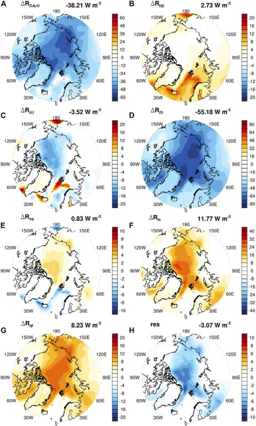
Huang et al.                                                                                                                              Nonlinear Radiative Feedback

    Often assumed in feedback analysis is linear additivity of the         nonlinear effects compare to the linear effects in terms of
radiative effects of different feedback variables. For instance, the       magnitude and pattern. We note that in this paper we are not
widely adopted kernel method (Soden and Held 2006) measures                concerned with how the changes in these variables are resulted,
the radiation change caused by a feedback variable (X) by                  which if nonlinearly related to the surface warming may also cause
                                                      zR
multiplying a pre-calculated radiative kernel (zX        ) with the        nonlinearity in climate feedbacks, but focus on how their changes,
climate response (dX). Due to its simple concept and                       as projected by the GCM, lead to nonlinear changes in the TOA
computational efficiency, a large number of studies have been               longwave (LW) and shortwave (SW) radiation energy fluxes. In the
conducted using this method (e.g., Soden and Held 2006; Zelinka            following sections, we will define, demonstrate and discuss the
et al., 2012; Vial et al., 2013; Zhang and Huang, 2014) and pre-           various feedback effects of interest in order.
computed kernels based on different atmospheric datasets,
including climate models, reanalyses and satellite data (e.g.,
Soden et al., 2008; Yue et al., 2016; Huang et al., 2017).                 METHOD: FEEDBACK DEFINITIONS
    The nonlinear effects, however, are often too large to ignore.
When individual feedback terms are independently measured,                 Here, we define a radiative feedback as the (partial) radiation
such as the non-cloud feedbacks in the clear-sky case in the               change, in the units of W m−2, due to one or multiple feedback
kernel method, the ignored nonlinear effects may lead to a                 variables. This should be distinguished from a feedback
non-closure of the radiation budget, i.e., the sum of the                  parameter, which is normalized by surface temperature change
individual terms cannot reproduce the overall radiation                    and is in the units of W m−2 K−1.
change (e.g., Huang 2013; Vial et al., 2013). In the Arctic,                  Consider the radiation field of interest, e.g., the TOA or surface
where climate perturbations are of large magnitudes, e.g., in              radiation flux, as a function of the feedback variables:
the case of sea ice melt, the non-closure issue is especially              R  R(x, y, z), where the letters (x, y, z) are generic notations
noticeable (e.g., Shell et al., 2008; Block and Mauritsen 2013;            of the feedback variables. The total radiation change in a given
Zhu et al., 2019). Besides the large perturbations in surface              climate change scenario can thus be expressed by a Taylor
albedo, the Arctic is also noted for its strong and unique lapse           series as
rate (e.g., Pithan and Mauritsen 2014) and cloud (e.g., Kato
                                                                                   ΔR(x,y,z)  Rx2 , y2 , z2  − Rx1 , y1 , z1
et al., 2006) feedbacks. It should be noted that although some
methods exhibit a seemingly good radiation closure, the                                zR     zR   zR
                                                                                         Δx + Δy + Δz                   univariate linear effects
                                                                                       zx     zy   zz
nonlinear effects are not treated but hidden in the feedback
term(s) measured as a residual, e.g., the cloud feedback term in                   1 zR  2
                                                                                               zR     2
                                                                                                      2 zR           2
                                                                                  +  2 (Δx)2 + 2 Δy + 2 (Δz)2                     univariate nonlinear effects
                                                                                   2 zx        zy       zz
the typical kernel method, including the adjusted cloud
radiative forcing (aCRF) technique (Shell et al., 2008; Soden                          z2 R          z2 R          z2 R
                                                                                  +2        ΔxΔy + 2      ΔyΔz + 2      ΔxΔz multivariate nonlinear effects
                                                                                       zxzy          zyzz          zxzz
et al., 2008).
                                                                                  + OΔ3
    Although the existence of the nonlinear effects has been
                                                                                                                                                                      (1)
recognized (e.g., Zhang et al., 1994; Colman et al., 1997), their
impacts were seldom isolated and quantified. Some recent works              where the subscripts 1 and 2 denote two different climate states, e.g.,
have specifically addressed the nonlinearity issue in the radiative         those before and after quadrupling CO2 (noted as 1xCO2 and 4xCO2,
feedback analysis. Zhu et al. (2019) for the first time used a neural       respectively from now on); such terms as Δx  x2 − x1 denote the
network model (a nonlinear diagnostic method without linearity             climate responses. The terms on the righthand side of Eq. (1) illustrate
assumption) to assess the radiative feedbacks and identified a few          three types of radiative effects that we aim to elucidate here:
strong nonlinear effects, including a strong cloud-water vapor
coupling effect in the tropical climate variations and a strong            1) The univariate linear effects, such as zR
                                                                                                                     zx Δx, which we denote
nonlinear dependence of radiation flux on the surface albedo.                  as ΔRx ;
                                                                           2) The univariate nonlinear effects, such as 12 zzxR2 (Δx)2 , which we
                                                                                                                             2
Using Partial-Radiative-Perturbation (PRP) experiments and
brute-force radiation model-based computations, Huang and                     denote as ΔRxx ;
                                                                                                                                 z2 R
Huang (2021) verified the cloud-water vapor coupling effect and             3) The multivariate nonlinear effects, such as zxzy        ΔxΔy, which
offered an analytic estimation of this effect on the longwave                 we denote as ΔRxy .
radiation. Shakirova and Huang (2021) advanced the neural
network model of Zhu et al. and demonstrated its advantages                   To avoid confusion, we denote a univariate feedback, i.e., the
particularly for quantifying the albedo feedback.                          overall radiation change due to a single variable, as ΔR(x) , which
    In this paper, we aim to give an overview of the nonlinear             consists of both univariate linear (ΔRx ) and univariate nonlinear
radiative feedback effects in Arctic climate change. Based on a            (ΔRxx ) effects:
heuristic climate change scenario of broad interest: the abrupt
quadrupling of atmospheric CO2 (4xCO2), we investigate how the                                ΔR(x)  Rx2 , y1 , ... − Rx1 , y1 , ...
nonlinear radiative effects arise from the univariate and
                                                                                                     zR      1 z2 R                                                   (2)
multivariate variations of the feedback variables, such as                                             Δx +       (Δx)2 + OΔ3
                                                                                                     zx      2 zx2
atmospheric and surface temperature (t), water vapor (q),
surface albedo (a) and cloud (c), and measure how the                                                       ΔRx + ΔRxx

Frontiers in Earth Science | www.frontiersin.org                       2                                                 August 2021 | Volume 9 | Article 693779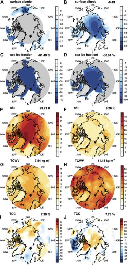
Huang et al.                                                                                                                  Nonlinear Radiative Feedback

Equation (2) is written following the PRP concept (Wetherald and                 which, as shown in the above expansion, effectively includes
                                                                                                                           z2 R
Manabe 1988) and measures the univariate feedbacks by simply                     nonlinear coupling effects such as 12 zxzy     ΔxΔy in δR(x) . When
evaluating the radiation flux twice: first with an unperturbed profile,             individual feedbacks are evaluated this way, their sum can better
R(x1 , y1 , ...), and then perturbing x only, R(x2 , y1 , ...). Note that        reproduce the overall radiation change, i.e., achieving a better
other unperturbed independent variables than y are omitted in these              radiation closure. However, it should be noted these "individual"
expressions. If not otherwise stated, unspecified independent                     feedbacks δR(x) differ from the univariate feedbacks ΔR(x) as δR(x)
variables all take the unperturbed values when the radiation fluxes               contains coupling effects. To disclose these coupling effects, we adopt
are evaluated in the following. The evaluation of the radiation fluxes            the one-sided formulations as exemplified by Eq. 2, Eq. 3, and Eq. 4
can be done using a physical model, i.e., a radiative transfer model
(RTM) (Huang and Huang 2021), or a statistical model, e.g., a neural
network model that emulate the radiation fluxes (Zhu et al., 2019).               RESULTS
   Similarly, a bivariate feedback can be expressed as:
                                                                     In this paper, we use the climate change in an abrupt 4xCO2
                       ΔR(x,y)  Rx2 , y2  − Rx1 , y1            experiment of CESM (Wang and Huang, 2020) to provide a
                                                                     context   for examining the linear and nonlinear radiative
  zR      zR     1 z2 R          1 z2 R          z2 R
     Δx + Δy +         (Δx) 2
                               +        Δy
                                             2
                                               +      ΔxΔy + OΔ 3
                                                                    feedbacks. As illustrated in Figure 1 for a few selected
  zx       zy    2 zx2           2 zy2           zxzy                variables, this scenario represents strong perturbations in the
                ΔRx + ΔRy + ΔRxx + ΔRyy + ΔRxy                      Arctic climate, including reduction in surface albedo due to sea
                                                             (3)     ice melt, surface warming and atmospheric moistening. The
                                                                     feedback quantifications presented in the following are based
From Eq. 2 and Eq. 3, the bivariate coupling effect ΔRxy can be      on the two months exemplified in Figure 1 if not
obtained as                                                          otherwise noted.
                   ΔRxy  ΔR(x,y) − ΔR(x) − ΔR(y)
                                                                       (4)       Univariate Linear Effects
            Rx2 , y2  − Rx2 , y1  − Rx1 , y2  + Rx1 , y1
                                                                                 The univariate linear effect ΔRx can be measured, following its
    Based on the above equations and following Huang and Huang                   definition, by multiplying the radiative linear sensitivity kernel
(2021), we evaluate the radiation fluxes and isolate the respective               Kx  zR
                                                                                       zx with the climate response Δx: Rx  Kx Δx. This is the core
feedback effects (ΔRx , ΔRxx , ΔRxy , etc.), using the Rapid Radiative           idea of the kernel method (Soden et al., 2008). The kernels are
Transfer Model (RRTM, Mlawer et al., 1997). Using this RTM, the                  usually pre-computed, again, following the PRP idea, by
TOA and surface radiation fluxes are computed offline from                         prescribing small perturbations to the individual variables, e.g.,
instantaneous atmospheric profiles generated by the Community                     1-K in atmospheric and surface temperatures, several percent
Earth System Model, CESM1.2, in a quadrupling CO2 experiment                     change in water vapor concentration, or 0.01 increment of surface
(Wang and Huang, 2020). More details of the flux computation can be               albedo (e.g., Shell et al., 2008):
found in Huang and Huang (2021); we note that the radiative transfer                                 ΔR0 Rx1 + Δx0 , y1  − Rx1 , y1
computations, including the PRP computations, are based on                                    Kx                                                     (6)
                                                                                                     Δx0             Δx0
instantaneous (3-hourly, as opposed to monthly mean) profiles at
the original horizontal resolutions (1.9 ° × 2.5 °) of the CESM and then         so that the kernel method is in essence to scale up the radiation
averaged monthly or annually in all the results presented in the                 change due to an infinitesimal (small) perturbation, R0 , to
following section.                                                               estimate the radiation change due to a finite (large) perturbation:
    Note that we use a one-sided PRP, starting with the
                                                                                                                             Δx
unperturbed climate and then prescribing the change(s) in the                                           ΔRx  Kx Δx  ΔR0                              (7)
variables of interest, to define feedbacks, i.e., how much radiation                                                          Δx0
change is caused by the change of the feedback variable(s) of                        It is worth noting that when defining and applying the kernels,
concern. Some studies opt to use two-sided perturbations (e.g.,                  it is advisable to choose a scaling scheme appropriate to the
Colman and McAvaney 1997). In contrast to Eq. (2), one may                       radiation dependency on the feedback variable. For instance, in
evaluate the feedback of x as                                                    the case of such greenhouse gases as carbon dioxide and water
            1                                                                    vapor, their radiative effects are logarithmically dependent on
     δR(x)  Rx2 , y1  − Rx1 , y1  + Rx2 , y2  − Rx1 , y2              their concentrations (e.g., Bani Shahabadi and Huang., 2014), so
            2
            1 zR          zR            1⎢zR                                     that it is common to define the water vapor kernel with respect to
           ≈ ⎢⎡⎣    Δx +         Δx⎤⎥⎦ ≈ ⎡
                                         ⎣       Δx + ⎛⎝zR                       the change in the logarithm of the specific humidity,
            2 zx y1        zx y2        2 zx y1          zx y1                                  ΔR0
                                                                                 i.e., Kq  Δ(ln(q)) 0
                                                                                                       , or, in an approximate form, using the
                                                                                                                                          ΔR0
                   z zR     ⎠Δx                                                  fractional change in q in the denominator, i.e., Kq  (Δq/q)   . As
               +       Δy⎞                                                     shown by Figure 2, using the logarithmic scaling scheme, the
                                                                                                                                              0
                   zy zx y1
                                                                                 radiation change caused by water vapor perturbations, even when
                   zR 1 z2 R                                                     the perturbations are of large magnitudes (about 200% increase of
                    +       ΔxΔy                                      (5)
                   zx 2 zxzy                                                     TCWV), can be well approximated according to Eq. (7).

Frontiers in Earth Science | www.frontiersin.org                             3                                      August 2021 | Volume 9 | Article 693779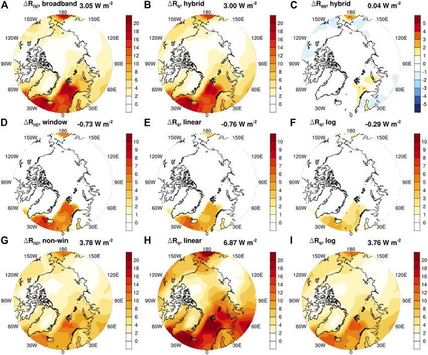
Huang et al.                                                                                                                                    Nonlinear Radiative Feedback

  FIGURE 1 | Changes in climate variables in the 4xCO2 experiment, exemplified by two months a January (left column) and a June (right column). (A,B) Suface
  albedo; (C,D) sea ice fraction; (E,F) surface skin temperature; (G,H) column-integrated water vapor; (I,J) total cloud fraction. The numbers on the upper right corner of
  each panel are the Arctic mean values, averaged over the latitude range of 70–90°N. Shaded in grey are regions with no data, for instance, due to no solar insolation to
  infer surface albedo in (A).

Frontiers in Earth Science | www.frontiersin.org                                      4                                             August 2021 | Volume 9 | Article 693779
Huang et al.                                                                                                                                   Nonlinear Radiative Feedback

  FIGURE 2 | Clear-sky univariate water vapor LW feedback. (A) RTM-computed (truth) overall univariate feedback, ΔR(q) ; (B) kernel-estimated univriate linear
  feedback, ΔRq , based on logarithmic scaling; (C) the residual (A–B), i.e., the univariate nonlinear feedback, ΔRqq . Shown here is the clear-sky TOA LW radiation flux
  change due to the water vapor change in January in the 4xCO2 experiment (as illustrated in Figure 1E). The kernel used in (B) is computed from the GCM instantaneous
  atmospheric profiles of the same month and is not subject to the bias discussed in Eq. 8.

  FIGURE 3 | All-sky univariate surface albedo SW feedback. (A) RTM-computed (truth), ΔqR(a) ; (B) kernel-estimated univariate linear feedback, ΔRa ; and (C) the
  residual (A–B), i.e., the univariate nonlinear term ΔRaa . Shown here is the all-sky TOA SW radiation flux change due to the surface albedo change in June in the 4xCO2
  experiment (as illustrated in Figure 1B).

    The validations against RTM-computed truth in Figures 2, 3                                     zR
                                                                                          ΔRx′                   Δx
show that the non-cloud univariate radiative feedbacks ΔR(x) ,                                     zx x′1,y′1,z′1
even in the case of large climate perturbations, can be reasonably
approximated by the linear term ΔRx . This is the basis of the                             ⎝   zR            z2 R                z2 R                  z2 R                 ⎠Δx
                                                                                          ≈⎛                + 2            dx′ +                 dy′ +                 dz ′ ⎞
kernel method (Soden et al., 2008). Nevertheless, the biases,                                  zx x1 ,y1 ,z1 zx x1 ,y1 ,z1       zxzy x1 ,y1 ,z1       zxzz x1 ,y1 ,z1
i.e., the univariate nonlinear effects ΔRxx may amount to non-
                                                                                           ΔRx + bias
negligible extent: in the case of the univariate water vapor
feedback and the surface albedo feedback, the biases can                                                                                                                   (8)
amount to more than 10% in terms of Arctic mean (averaged                                   Equation (8) shows that the bias can be considered one type of
over 70–90°N).                                                                           nonlinear effect in that it, like the nonlinear effects analyzed
    It should be cautioned that the kernel itself has a dependency
                                                                                         below, results from the nonlinear dependency of the radiation on
on the atmospheric conditions (x, y, z, . . . ) and such dependency                                                         z2 R
should be recognized when interpreting the kernel-diagnosed                              the feedback variables (e.g., zxzy      ). For the simplicity of the
feedbacks. The kernels appropriate to evaluating the linear                              expressions, we omit the notation (...)|x1 ,y1 ,z1 in the following,
feedbacks in Eq. 1, Eq. 2, and Eq. 3, and used to compute                                where the conditioned states can be inferred from the context.
ΔRq in Figure 2 and ΔRa in Figure 3, are computed from the                                  The magnitude of the feedback bias caused by kernel bias is
GCM atmopsheric profiles in the unperturbed (1xCO2) climate,                              proportional to the discrepancies in the atmospheric states
                                                                                         (dx′ , dy′ , and dz ′ in Eq. (8)), which may introduce noticeable
i.e., Kx  zR
           zx                , where (x1 , y1 , z1 ) denotes the 1xCO2 climate. If
                x1 ,y1 ,z1                                                               quantitative differences in the kernels. For example, one may
computed from different atmospheric states, the kernel values                            see from Fig. S3 of Huang et al. (2017), as well as the
may quantitatively differ (e.g., see the kernel comparisons in                           discussions of Sanderson and Shell (2012), the temperature
Huang et al., 2017; Smith et al., 2020 and others). If a kernel                          kernel discrepancies due to the ubiquitous discrepancies in
computed from a different atmospheric state (x1′ , y1′ , z1′ ) is used to                the cloud distribution in different atmospheric datasets used
measure the linear feedback, a bias is resulted:                                         for kernel computation. Here, as a sanity check, we recalculate

Frontiers in Earth Science | www.frontiersin.org                                     5                                            August 2021 | Volume 9 | Article 693779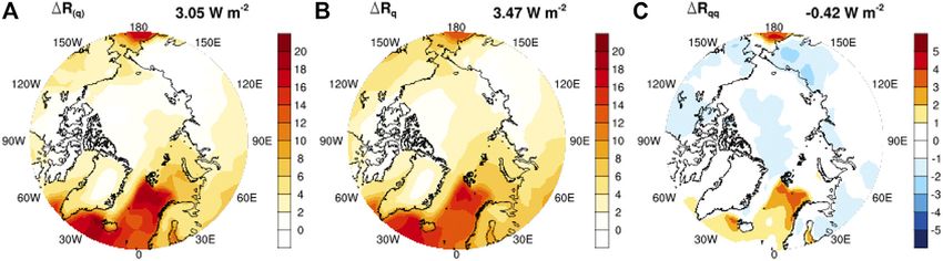
Huang et al. Nonlinear Radiative Feedback
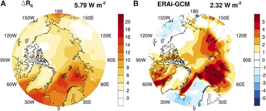
FIGURE 4 | Clear-sky water vapor feedback bias due to kernel bias. (A) Like Figure 2B, but using the kernels computed from different atmospheric profiles (Huang
et al., 2017); (B) Bias compared to Figure 2B.
the Arctic mean clear-sky water vapor feedback shown in although this nonlinearity is weak at the terrestrial
Figure 2 using the clear-sky kernels of Huang et al. (2017) and temperatures. Based on the Stefan-Boltzmann Law,
obtain an Arctic mean ΔRq of 5.79 W m−2 (Figure 4). This,
compared to the RTM-computed truth value of 3.05 W m−2 , R σt 4 (9)
representes a 90% bias and is much larger than the bias when −8 −2 −4
Given the constant σ 5.67 × 10 W m K , one may find
the correct (GCM 1xCO2 climate based) kernels are used that the nonlinear effect zztR2 is only about 1% of the linear effect zR
2
zt ,
(3.47 W m−2 , as shown by Figure 2B). The results indicates for a 1-K perturbation around the equivalent blackbody
that, contradictory to common belief, there may be large temperature of Earth (t 255K). Another cause of the
biases, especially in regional (e.g., Arctic) feedbacks, nonlinearity is the dependence of the gas absorptivity on the
resulting from kernel biases. temperature, which also has a minor impact (Huang et al., 2007).
Lastly, we note that cloud feedback is difficult, if not impossible, This explains why the temperature feedback in the case of large
to be approximated by linear kernels. This is because cloud perturbations can still be very well approximated by the linear
variations involve multiple radiative properties, including cloud kernels (not shown).
fraction, droplet concentration and size distribution, etc., each of
which may experience large, discrete perturbations and strongly Water Vapor
affect the radiative sensitivity to each other. The cloud radiative The univariate water vapor feedback is generally well
effects measured in the cloud property histogram method (Zelinka estimated when the logarithmic scaling scheme is used,
et al., 2012) illustrate how the radiative sensitivity to cloud varies although Figure 2C shows that the bias (i.e., the univariate
strongly with the cloud properties. Among other issues, a notable nonlinear effect, ΔRqq ) can be non-negligible. A notable
challenge is the vertical masking effect: for instance, the increase of reason that causes the feedback to deviate from the
upper-level clouds greatly reduces the sensitivity of the TOA fluxes logarithmic behavior is the unsaturated atmospheric
to the lower-level clouds. absorption in the mid-infrared window around 10 μm
In summary, the non-cloud univariate feedbacks in general wavelength. Here, the surface emission strongly
can be approximated well by the kernel method, although one contributes to the OLR and thus the water vapor feedback
should be mindful about the biases introduced by kernel cannot be interpreted simply as the elevation of the
discrepancies. One most noticeable univariate nonlinear effect atmospheric emission level, which gives rise to the
in the Arctic is the surface albedo feedback. We further analyze logarithmic dependence (Bani Shahabadi and Huang.,
this and other nonlinear effects in the following subsections. 2014). Figure 5 suggests that the water vapor feedback
estimation may be improved if different scaling schemes
Univariate Nonlinear Effects are used for different spectral bands: logarithmic in the
Because radiative transfer is a complex nonlinear process (e.g., see absorption bands (where atmospheric optical depth is
Goody and Yung 1989), atmospheric radiation fluxes generally large) and linear in the window bands (where optical
have a nonlinear dependency on the feedback variables and thus depth is small):
the univariate nonlinear effects generally exist.
ΔR(q) Kqlog Δlnq + Kqlin Δq (10)
Temperature
log
With regard to the univariate temperature feedback, a well- where the logarithmic kernel Kq accounts for the logarithmic
recognized cause of the nonlinearity is the Planck function, response of the radiation flux in the absorption bands to water
Frontiers in Earth Science | www.frontiersin.org 6 August 2021 | Volume 9 | Article 693779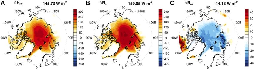
Huang et al.                                                                                                                         Nonlinear Radiative Feedback

  FIGURE 5 | Spectral breakdown of the clear-sky univariate water vapor feedback. (A) RTM-computed (truth) broadband univariate feedback, ΔR(q) ; (B) kernel-
  diagnosed broadband feedback, ΔRq , using the hybrid scaling (Eq. 10); (C) residual, ΔRqq . (D–F) Window band (700–1,180 cm−1) feedback, computed by RTM and
  estimated by linear and logarithmic scaling. (G–I) Like (D–F), but for the non-window (absorption) bands.

vapor perturbation and the linear kernel Kqlin accounts for the                                                  zap   τ2
                                                                                                                                                           (12)
linear response in the window band. Further research is required                                                 za (1 − ra)2
to develop and validate a global hybrid kernel set.
                                                                                    That the radiative sensitivity to surface albedo continuously varies
Surface Albedo                                                                      with the albedo value makes it difficult for any linear methods
The univariate surface albedo feedback shows especially strong                      such as the kernel method to accurately measure the albedo
nonlinear dependence on the surface albedo a (Figure 6). This is                    feedback. It is interesting to notice from Eq. (12) that the radiative
because the multiple scattering of radiation between the surface                    sensitivity decreases with a. This means that if the surface albedo
and atmosphere renders a nonlinear dependency of planetary                          kernel is computed with relatively larger albedo values under the
albedo on surface albedo. Following Stephens et al. (2015), the                     unperturbed climate (1xCO2), it will overestimate the univariate
planetary albedo ap can be expressed as                                             albedo feedback in a warming scenario (4xCO2). This is clearly
                                                                                    seen from Figure 6. If the kernel method is used to estimate the
                                            aτ 2                                    feedback when sea ice completely melts, the intercepts on y-axis
                                ap  r +                                 (11)       indicate the overestimate can be serveral dozens of W m−2. This
                                           1 − ra
                                                                                    overestimation issue was also noted in the previous studies (e.g.,
   Here r and τ denote atmospheric reflectance and                                   Block and Mauristen 2013; Zhu et al., 2019). It is also interesting
transmittance respectively; they are related as τ + r + ε  1,                      to notice that although the analytical model qualitatively captures
where ε denotes atmospheric absorptivity. This relation means                       the change of radiative sensitivity to albedo, it does not accurately
that ap and thus the net shortwave radiation flux at TOA has a                       predict it. The neural network method proposed by Zhu et al.
nonlinear dependency on a:                                                          (2019) and Shakirova and Huang (2021) may be better suited for

Frontiers in Earth Science | www.frontiersin.org                                7                                         August 2021 | Volume 9 | Article 693779
Huang et al. Nonlinear Radiative Feedback
Due to large computational expenses of the brute-force RTM-
based feedback calculation, we base our discussions on two
representative months in the 4xCO2 experiment: January
(winter) for the longwave feedbacks and June (summer) for
the shortwave feedbacks, because the two types of feedbacks are
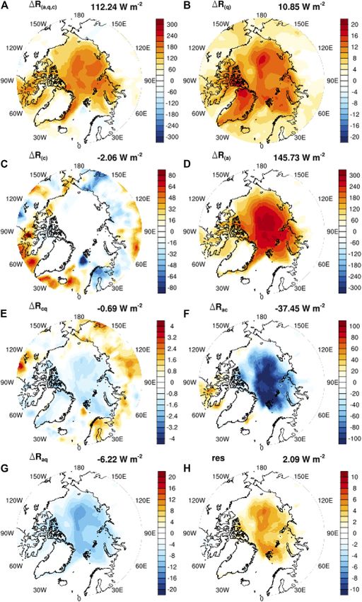
the most prominent in the two respective seasons. Figures 7,8 show
the radiative feedbacks corresponding to the changes in the feedback
variables illustrated in Figure 1. Table 1 summarizes their Arctic
mean values. These results disclose two strongest multivariate
feedback effects in the Arctic: the coupling effect between
temperature and cloud, ΔRtc , in the longwave and the coupling
effect between albedo and cloud, ΔRac , in the shortwave.
In the longwave, we find that the multivariate (bivariate)
feedback is dominated by the coupling effect between
temperature and cloud, ΔRtc . The pattern of this coupling
effect resembles, but strongly offsets, the univariate
temperature feedback, ΔR(t) , which is the dominant feedback
that controls the overall LW feedback in the Arctic. This coupling
effect can be explained by a simple analytical model. Consider a
single-layer atmosphere, with temperature ta and emissivity
(absorptivity) ε, and assume the surface to be a blackbody
with temperature ts :
OLR (1 − ε)σts4 + ε σta4 (13)
Hence, the coupling effect ΔOLRtc is found to be
dε
ΔOLRtc 4σta3 Δta − ts3 Δts Δc (14)
dc
Because the warming in the Arctic is capped in near-surface
layers, Δta < < Δts . This leads to reduction in OLR, offseting the
increase of OLR by temperature warming. The coupling effect
FIGURE 6 | All-sky univariate surface albedo SW feedback between temperature and water vapor can be understood in the
corresponding to different albedo values. By perturbing the surface albedo to same way. Becaue water vapor affects OLR also by affecting the
values from 0 to 1, the TOA SW feedback is computed by three different atmospheric emissivity; the coupling effect ΔOLRtq is thus also
methods: RRTM-computed truth, kernel-estimation and the single-layer
analytical model (Eq. 11). The results are compuated based on one arbitrarily
affected by the factor (ta3 Δta − ts3 Δts ) in Eq. (14). Although this
chosen grid box at (78°W, 82°N), where the intial surface albedo is 0.85. nonlinear effect arises from the nonuniform vertical structure of
temperatuure warming and thus share the physical cause of the
temperature lapse rate feedback, this nonlinear effect should be
distinguished from the lapse rate feedback, which is part of the
the albedo feedback quantification and deserves further univariate temperature feedback, ΔRt . Note that the sign of ΔRtc
development and more extensive validations. and ΔRcq is positive in Figure 7 because the fluxes are defined to
be downward positive.
Multivariate Nonlinear Effects In the shortwave, the dominant multivariate effect is found to
Besides the univariate nonlinear effects, Eq. (1) indicates that be the albedo-cloud coupling, which offsets the univariate albedo
multivariate nonlinear effects, represented by such terms as feedback. From the simple model described above (Eq. 11 and Eq.
z2 R
zxzy ΔxΔy, may also strongly contribute to the radiative flux 12, this can be understood as cloud-caused reduction in the
variations. Such terms are often referred to as the coupling atmospheric transmittance and thus reduction in the radiative
effects because they result from concerted variations of the senstivity to surface albedo.
involved variables; otherwise, if their covariance were small, It is interesting to note that the patterns of some coupling
the average of this term over time or region would be feedback effects are correlated with the change patterns of the
negligible. In reality, this necessary condition is usually met associated feedback variables. For example, the LW cloud-
because the variations of the feedback variables of concern temperature coupling effect is correlated with surface
tend to be strongly correlated. For instance, temperature temperature change, with a correlation coefficient of 0.86; the
warming and sea ice melt may expose more open water, LW cloud-water vapor coupling effect is correlated with total
which in turn leads to more evaporation, atmospheric water vapor (TCWV) at 0.62; the SW albedo-cloud coupling
humidity and cloudiness. effect is correlated with the surface albedo change at 0.89. Such
Frontiers in Earth Science | www.frontiersin.org 8 August 2021 | Volume 9 | Article 693779Huang et al. Nonlinear Radiative Feedback FIGURE 7 | All-sky LW feedback effects in January. Units: W m−2. Shown here are the total and component all-sky feedbacks in the 4xCO2 experiment evaluated according to Eq. 2, Eq. 3, and Eq. 4 by using an RTM. t: atmospheric and surface temperatures; q: atmospheric water vapor; c: cloud; a: surface albedo; res: residual. The Arctic mean values are noted on the top right corner of each panel. Frontiers in Earth Science | www.frontiersin.org 9 August 2021 | Volume 9 | Article 693779
Huang et al.                                                                                                              Nonlinear Radiative Feedback

  FIGURE 8 | Like Figure 7, but for the all-sky SW feedback effects in June. Units: W m−2.

relation suggests that it may be possible to estimate these                          cloud-water vapor coupling effect and found it to be the
nonlinear effects using analytical or statistical models. Huang                      dominant multivariate longwave feedback effect in the
and Huang (2021) used such an model to explain the                                   tropics. Although this coupling effect is not as strong

Frontiers in Earth Science | www.frontiersin.org                                10                              August 2021 | Volume 9 | Article 693779
Huang et al.                                                                                                                               Nonlinear Radiative Feedback

TABLE 1 | Arctic mean all-sky feedbacks in the 4xCO2 experiment for the two selected months. Units: W m-2. Area-weighted averages are taken for the region 70–90°N.
Two sets of radiative kernels have been used to measure the univariate linear feedbacks: Ker1 is computed from the GCM instantaneous profiles in this work and thus is
of no kernel bias; Ker2 is the kernel computed by Huang et al. (2017) from the ERA-interim reanalysis profiles, which leads to biases in diagnosed univariate feedback as
explained by Eq. 8.

LW              ΔR(t,q,c)          ΔR(t)           ΔR(q)           ΔR(c)           ΔRcq            Rtc            ΔRqt            res                     ΔTS (K)
(jan
                                                                                                                                                 Global             Arctic
                                                                                                                                                 mean               mean

RTM              −38.21            −55.18           2.73           −3.52           0.83           11.77           8.23           −3.07            7.95              29.71
—                  —                ΔRt             ΔRq             ΔRpc            —              —               —              —
Ker1               —               −48.98           3.08            7.68            —              —               —              —
Ker2               —               −44.53           5.35            0.97            —              —               —              —

SW                ΔR(a,q,c)          ΔR(a)          ΔR(q)           ΔR(c)           ΔRcq            ΔRac            ΔRqa           res                    ΔTS (K)
(Jun.)
                                                                                                                                                 Global             Arctic
                                                                                                                                                 mean               mean

RTM                112.24           145.73          10.05          −2.06            −0.69          −37.45           −6.22          2.09           6.97              9.20
—                    —               ΔRa             ΔRq             ΔRpc            —               —               —              —
Ker1                 —              159.85          12.26          −59.88            —               —               —              —
Ker2                 —              117.04           8.14           12.95            —               —               —              —

compared to the temperature-related coupling effects in the Arctic,                     climate are used to quantify the albedo feedback in a warming
we find that adopting the same estimation method of Huang and                            climate (Figure 3; Table 1).
Huang, 2021, Eq. 19 and using a parameter value appropriate to the                          2) The bivariate surface albedo-cloud coupling effect in the
Arctic (A  0.04 kg−1 m2), we can very well predict the cloud-water                     shortwave. This effect is attributable to the masking effect of cloud
vapor coupling effect (spatial correlation  0.99, RMSE  0.41 W                        increase that damps the radiative sensitivity to surface albedo. This
m−2). Future works are warranted to identify methods for                                effect is the most prominent in the summer when solar insolation is
explaining and predicting the other coupling effects.                                   strong, as illustrated by Figure 8 for the month of June.
   Lastly, for comparison, we include in Table 1 the respective                             3) The multivariate temperature-cloud feedback in the
feedbacks analyzed from the kernel method, i.e., the univariate                         longwave. This effect is attributable to the fact that the
linear effects for non-cloud feedbacks and the cloud feedback                           Arctic warming is much stronger at and near the surface
(ΔRpc ) obtained as a residual of total radiation change                                than in the upper air, which leads to a damping effect on
decomposition. Besides the biases in the univariate feedbacks                           the temperature feedback. This nonlinear effect should be
as noted above, it is worth noting that the kernel-based                                distinguished from the temperature lapse rate feedback and
estimations may also greatly bias the cloud feedback, mainly                            is found to be the strongest in the winter as illustrated by
due to its negligence of the coupling effects.                                          Figure 7 for the month of January.
                                                                                            4) Although the univariate water vapor feedback largely scales
                                                                                        logarithmically with water vapor changes, it is found that the relation
CONCLUSIONS AND DISCUSSIONS                                                             deviates from the logarithmic scaling, especially in the window band.
                                                                                        This is due to the unsaturated atmospheric absorption in this band
In this paper, we present an overview of the nonlinear effects in both                  and suggests that a hybrid scaling method as proposed by Eq. (10)
longwave and shortwave radiative feedbacks in the CO2-driven Arctic                     may improve the accuracy of the kernel-diagnosed water vapor
warming. Based on brute-force radiation model calculations we                           feedback (compare Figure 2C and Figure 5C).
disclose the most prominent nonlinear feedback effects and based                            It should be noted that the large nonlinear effects discovered here is
on simple analytical models we offer explanations of their physcial                     not limited to the 4xCO2 experiment. As shown by Huang and Huang
causes. Although the presentation and discussion are focused on the                     (2021) for the longwave feedbacks and Shakirova and Huang (2021)
Arctic feedbacks, the diagnostic framework (Eq. 1) and the theoretical                  for the shortwave feedbacks, similar, strong nonlinear effects exist even
explanations are applicable to global feedback analyses.                                also interannual climate variations. It is noted that the nonlinear effects
    We identify these important nonlinear feedback effects:                             may quantitatively differ in different forcing experiments, thus
    1) The univariate nonlinear effect in the surface albedo feedback                   requiring them to be assessed more comprehensively in future work.
in the shortwave. This nonlinearity can be understood from a                                The strong nonlinear effects as disclosed here call into question
simple analytical model [Eq. (11)] that accounts for the coupling,                      the accuracy of linear methods currently used in the feedback
due to multiple-scattering, between the surface and atmosphere                          analysis. Nonlinear methods are needed to improve the accuracy
(clouds). This coupling makes the radiative sensitivity to surface                      of feedback quantificaiton when RTM-based PRP experiments are
albedo decrease with the surface albedo value (Figure 6). Because                       not feasible due to its forbidding computational demands. Especially
of this effect, it generally leads to an overestimate of the surface                    in need are replacement of the linear kernels for the surface albedo
albedo feedback when albedo kernels computed from the current                           feedback and cloud feedback quantification. Although a handful of

Frontiers in Earth Science | www.frontiersin.org                                   11                                           August 2021 | Volume 9 | Article 693779
Huang et al. Nonlinear Radiative Feedback
studies have touched this topic, for instance, using quadratic fitting AUTHOR CONTRIBUTIONS
(Colman et al., 1997), histogram (Zelinka et al., 2012) and neural
network (Zhu et al., 2019) methods, this challenging problem YH designed the research and wrote the paper. HH conducted the
demands devoted research programs to further develop, test and longwave feedback analysis and AS conducted the shortwave
mature the candidate methods. feedback analysis.
DATA AVAILABILITY STATEMENT ACKNOWLEDGMENTS
The datasets presented in this study can be found in online We thank Tim Merlis, Ivy Tan, Patrick Taylor and two reviewers,
repositories. The names of the repository/repositories and accession whose comments helped improve this paper. We acknowledge
number(s) can be found below: The CESM codes can be downloaded grants from the Natural Sciences and Engineering Research
from National Center for Atmospheric Research (NCAR) website Council of Canada (RGPIN-2019-04511) and from the Fonds
(http://www.cesm.ucar.edu/models/cesm1.2/). The RRTM code can de recherche du Québec—Nature et technologies (2021-PR-
be downloaded at http://rtweb.aer.com/rrtm_frame.html. 283823).
Soden, B. J., Held, I. M., Colman, R., Shell, K. M., Kiehl, J. T., and Shields, C. A.
REFERENCES (2008). Quantifying Climate Feedbacks Using Radiative Kernels. J. Clim. 21
(14), 3504–3520. doi:10.1175/2007jcli2110.1
Bani Shahabadi, M., and Huang, Y. (2014). Logarithmic Radiative Effect of Water Vial, J., Dufresne, J.-L., and Bony, S. (2013). On the Interpretation of Inter-model
Vapor and Spectral Kernels. J. Geophys. Res. Atmos. 119 (10), 6000–6008. Spread in CMIP5 Climate Sensitivity Estimates. Clim. Dyn. 41 (11-12),
doi:10.1002/2014jd021623 3339–3362. doi:10.1007/s00382-013-1725-9
Block, K., and Mauritsen, T. (2013). Forcing and Feedback in the MPI-ESM-LR Wang, Y., and Huang, Y. (2020). The Surface Warming Attributable to
Coupled Model under Abruptly Quadrupled CO2. J. Adv. Model. Earth Syst. 5 Stratospheric Water Vapor in CO2-caused Global Warming. J. Geophys.
(4), 676–691. doi:10.1002/jame.20041 Res. Atmospheres 125, e2020JD032752. doi:10.1029/2020JD032752
Colman, R. A., Power, S. B., and McAvaney, B. J. (1997). Non-linear Climate Wetherald, R. T., and Manabe, S. (1988). Cloud Feedback Processes in a General
Feedback Analysis in an Atmospheric General Circulation Model. Clim. Dyn. Circulation Model. J. Atmos. Sci. 45 (8), 1397–1416. doi:10.1175/1520-
13 (10), 717–731. doi:10.1007/s003820050193 0469(1988)0452.0.co;2
Colman, R., and McAvaney, B. J. (1997). A Study of General Circulation Model Yue, Q., Kahn, B. H., Fetzer, E. J., Schreier, M., Wong, S., Chen, X., et al. (2016).
Climate Feedbacks Determined from Perturbed SST Experiments. J. Geophys. Observation-Based Longwave Cloud Radiative Kernels Derived from the
Res. 102, 19 383–419. doi:10.1029/97jd00206 A-Train. J. Clim. 29, 2023–2040. doi:10.1175/JCLI-D-15-0257.1
Huang, H., and Huang, Y. (2021). Nonlinear Coupling between Longwave Zelinka, M. D., Klein, S. A., and Hartmann, D. L. (2012). Computing and
Radiative Climate Feedbacks. J. Geophys. Res. Partitioning Cloud Feedbacks Using Cloud Property Histograms. Part I:
Huang, Y. (2013). On the Longwave Climate Feedbacks. J. Clim. 26 (19), Cloud Radiative Kernels. J. Clim. 25 (11), 3715–3735. doi:10.1175/jcli-d-11-
7603–7610. doi:10.1175/jcli-d-13-00025.1 00248.1
Huang, Y., Ramaswamy, V., and Soden, B. (2007). An Investigation of the Zhang, M. H., Hack, J. J., Kiehl, J. T., and Cess, R. D. (1994). Diagnostic Study of
Sensitivity of the clear-sky Outgoing Longwave Radiation to Atmospheric Climate Feedback Processes in Atmospheric General Circulation Models.
Temperature and Water Vapor. J. Geophys. Res. Atmospheres 112 (D5). J. Geophys. Res. 99 (D3), 5525–5537. doi:10.1029/93jd03523
doi:10.1029/2005jd006906 Zhang, M., and Huang, Y. (2014). Radiative Forcing of Quadrupling CO2. J. Clim.
Huang, Y., Xia, Y., and Tan, X. (2017). On the Pattern of CO2 Radiative Forcing 27 (7), 2496–2508. doi:10.1175/jcli-d-13-00535.1
and Poleward Energy Transport. J. Geophys. Res. Atmos. 122 (10), 578–593. Zhu, T., Huang, Y., and Wei, H. (2019). Estimating Climate Feedbacks Using a Neural
doi:10.1002/2017jd027221 Network. J. Geophys. Res. Atmos. 124 (6), 3246–3258. doi:10.1029/2018jd029223
Mlawer, E. J., Taubman, S. J., Brown, P. D., Iacono, M. J., and Clough, S. A. (1997).
Radiative Transfer for Inhomogeneous Atmospheres: RRTM, a Validated Conflict of Interest: The authors declare that the research was conducted in the
Correlated-K Model for the Longwave. J. Geophys. Res. 102 (D14), absence of any commercial or financial relationships that could be construed as a
16663–16682. doi:10.1029/97jd00237 potential conflict of interest.
Sanderson, B. M., and Shell, K. M. (2012). Model-Specific Radiative Kernels for
Calculating Cloud and Noncloud Climate Feedbacks. J. Clim. 25 (21), Publisher’s Note: All claims expressed in this article are solely those of the authors
7607–7624. doi:10.1175/jcli-d-11-00726.1 and do not necessarily represent those of their affiliated organizations, or those of
Shakirova, A., and Huang, Y. (2021). An Neural Network Model for Shortwave the publisher, the editors and the reviewers. Any product that may be evaluated in
Radiative Feedback Estimation. J. Geophys. Res. Atmosphere under this article, or claim that may be made by its manufacturer, is not guaranteed or
revision for. endorsed by the publisher.
Shell, K. M., Kiehl, J. T., and Shields, C. A. (2008). Using the Radiative Kernel
Technique to Calculate Climate Feedbacks in NCAR’s Community Copyright © 2021 Huang, Huang and Shakirova. This is an open-access article
Atmospheric Model. J. Clim. 21 (10), 2269–2282. doi:10.1175/2007jcli2044.1 distributed under the terms of the Creative Commons Attribution License (CC BY).
Smith, C. J., Kramer, R. J., and Sima, A. (2020). The HadGEM3-GA7.1 Radiative The use, distribution or reproduction in other forums is permitted, provided the
Kernel: the Importance of a Well-Resolved Stratosphere. Earth Syst. Sci. Data original author(s) and the copyright owner(s) are credited and that the original
Discuss 12, 2057–2068. doi:10.5194/essd-2019-254 publication in this journal is cited, in accordance with accepted academic practice.
Soden, B. J., and Held, I. M. (2006). An Assessment of Climate Feedbacks in Coupled No use, distribution or reproduction is permitted which does not comply with
Ocean-Atmosphere Models. J. Clim. 19 (14), 3354–3360. doi:10.1175/jcli3799.1 these terms.
Frontiers in Earth Science | www.frontiersin.org 12 August 2021 | Volume 9 | Article 693779You can also read