Inflation, B-mode, and String Theory Gary Shiu - University of Wisconsin & HKUST

Page created by Alan Gregory
 
CONTINUE READING
Inflation, B-mode, and String Theory Gary Shiu - University of Wisconsin & HKUST
Inflation, B-mode, and String Theory

               Gary Shiu
         University of Wisconsin & HKUST
Inflation, B-mode, and String Theory Gary Shiu - University of Wisconsin & HKUST
Inflation, B-mode, and String Theory

                   Gary Shiu
             University of Wisconsin & HKUST

          KEK-CPWS The 4th UTQuest Workshop
     KEK Theory Center Cosmophysics Group Workshop
                  “B-mode Cosmology”
Inflation, B-mode, and String Theory Gary Shiu - University of Wisconsin & HKUST
Based on:

•   F. Marchesano, GS, A. Uranga, “F-term Axion Monodromy
    Inflation,’' JHEP 1409, 184 (2014) [arXiv:1404.3040 [hep-th]].

    and some forthcoming work:

•   GS, W. Staessens, F. Ye, “Widening the Axion Window via Kinetic
    and Stuckelberg Mixings”, 1502.xxxxx [hep-th], to appear.
•   GS, W. Staessens, F. Ye, “Large Field Inflation from Axion
    Mixings”, 1502.xxxxx [hep-th], to appear.
•   J. Brown, I. Garcia-Etxebarria, F. Marchesano, GS, “Tunneling in
    Axion Monodromy Inflation”, in progress.
Inflation, B-mode, and String Theory Gary Shiu - University of Wisconsin & HKUST
Temperature Fluctuations
                                                 Planck Collaboration: The Planck mission
                                                                                                                                                                                                        Planck Collaboration: The Planck mission

                                                                                                                                                                                                                   Angular scale
                                                                                                                                                                          90        18                  1                         0.2                           0.1                     0.07
                                                                                                                                                            6000

                                                                                                                                                            5000                                                                                   PLANCK
                                                                                                                                                            4000

                                                                                                                                               D [µK2]
                                                                                                                                                            3000

                                                                                                                                                            2000

                                                                                                                                                            1000

                                                                                                                                                                 0
                                                                                                                                                                          2          10            50              500              1000             1500             2000              250
                                                                                                                                                                                                            Multipole moment,
 14. The SMICA CMB map (with 3 % of the sky replaced by a constrained Gaussian realization).                                                  Fig. 19. The temperature angular power spectrum of the primary CMB from Planck, showing a precise measurement of seven acoustic peaks,
                                                                                                                                              are well fit by a simple six-parameter ⇤CDM theoretical model (the model plotted is the one labelled [Planck+WP+highL] in Planck Collabora
                                                                                                                                              XVI (2013)). The shaded area around the best-fit curve represents cosmic variance, including the sky cut used. The error bars on individual po
                                                                                                                                              also include cosmic variance. The horizontal axis is logarithmic up to ` = 50, and linear beyond. The vertical scale is `(` + 1)Cl /2⇡. The measu
                                                                                                                                              spectrum shown here is exactly the same as the one shown in Fig. 1 of Planck Collaboration XVI (2013), but it has been rebinned to show be
                                                                                                                                              the low-` region.

       A nearly scale-invariant, adiabatic, Gaussian temperature                                                                                            90       18         1
                                                                                                                                                                                    Angular scale
                                                                                                                                                                                             0.2                   0.1
                                                                                                                                                                                                                                tected by Planck over the entire sky, and which therefore c
                                                                                                                                                                                                                                tains both Galactic and extragalactic objects. No polarization

       fluctuation spectrum as generically predicted by inflation
                                                                                                                                                   6000
                                                                                                                                                                                                                                formation is provided for the sources at this time. The PC
                                                                                                                                                   5000
                                                                                                                                                                                                                                di↵ers from the ERCSC in its extraction philosophy: more e↵
                                                                                                                                                                                                                                has been made on the completeness of the catalogue, without
                                                                                                                                                   4000                                                                         ducing notably the reliability of the detected sources, wher
                                                                                                                                              D [µK2]

             seems to be in excellent agreement with data.
                                                                                                                                                                                                                                the ERCSC was built in the spirit of releasing a reliable cata
                                                                                                                                                   3000                                                                         suitable for quick follow-up (in particular with the short-liv
                                                                                                                                                                                                                                Herschel telescope). The greater amount of data, di↵erent sel
                                                                                                                                                   2000
  15. Spatial distribution of the noise RMS on a color scale of 25 µK                                                                                                                                                           tion process and the improvements in the calibration and m
the SMICA CMB map. It has been estimated from the noise map                                                                                                                                                                     making processing (references) help the PCCS to improve
                                                                                                                                                   1000
ained by running SMICA through the half-ring maps and taking the                                                                                                                                                                performance (in depth and numbers) with respect to the pre
 -di↵erence. The average noise RMS is 17 µK. SMICA does not                                                                                             0                                                                       ous ERCSC.
duce CMB values in the blanked pixels. They are replaced by a con-                                                                                           2       10    50        500       1000         1500         2000
ined Gaussian realization.                                              Fig. 16. Angular spectra for the SMICA CMB products, evaluated over                                     Multipole moment,                                  The sources were extracted from the 2013 Planck frequen
Inflation, B-mode, and String Theory Gary Shiu - University of Wisconsin & HKUST
Two massless fields that are guaranteed to exist are:

ζ   Goldstone boson
    of broken time translations
                                     hij      graviton
Inflation, B-mode, and String Theory Gary Shiu - University of Wisconsin & HKUST
Two massless fields that are guaranteed to exist are:

    ζ        Goldstone boson
             of broken time translations
                                             hij      graviton
                                                                    expansion

    symmetry breaking
(       for slow-roll inflation)

E-modes:

B-modes:
Inflation, B-mode, and String Theory Gary Shiu - University of Wisconsin & HKUST
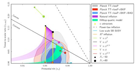
A distinguishing parameter is the tensor-to-scalar ratio r.

Many experiments including BICEP/KECK, PLANCK, ACT,
PolarBeaR, SPT, SPIDER, QUEIT, Clover, EBEX, QUaD…
  can potentially detect such primordial B-mode if r≾10-2.

LiteBIRD may even have the sensitivity to detect r ~ 10-3.

            M. Hazumi’s take home message:
           r ~ 10-2 in ~ 5 years, r~ 10-3 in 2020s
Inflation, B-mode, and String Theory Gary Shiu - University of Wisconsin & HKUST
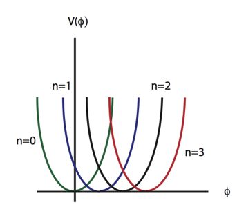
B-mode and Inflation

If primordial B-mode is detected, natural interpretations:
     ✦ Inflation took place

     ✦ The energy scale of inflation is the GUT scale
                              ⇣ r ⌘1/4
               Einf ' 0.75 ⇥              ⇥ 10 2 MPl
                                0.1
     ✦ The inflaton field excursion was super-Planckian
                              ⇣ r ⌘1/2
                            &           MPl               Lyth ’96
                                0.01
     ✦ Great news for string theory due to strong UV sensitivity!

       !
Assumptions in the Lyth Bound

single field

slow-roll

Bunch-Davies initial conditions

vacuum fluctuations
Assumptions in the Lyth Bound

single field

slow-roll
                                  Ashoorioon, Dimopoulos, Sheikh-Jabbari, GS
                                  Collins, Holman, Vardanyan
Bunch-Davies initial conditions   Aravind, Lorshbough, Paban

vacuum fluctuations
Assumptions in the Lyth Bound

single field

slow-roll
                                  Ashoorioon, Dimopoulos, Sheikh-Jabbari, GS
                                  Collins, Holman, Vardanyan
Bunch-Davies initial conditions   Aravind, Lorshbough, Paban

                                  Particle production during inflation
vacuum fluctuations
                                        can be a source of GWs

                                  Cook and Sorbo
                                  Senatore, Silverstein, Zaldarriaga
                                  Barnaby, Moxon, Namba, Peloso, GS, Zhou
                                  Mukohyama, Namba, Peloso, GS
Assumptions in the Lyth Bound

  single field

  slow-roll
                                                                    Ashoorioon, Dimopoulos, Sheikh-Jabbari, GS
                                                                    Collins, Holman, Vardanyan
      Bunch-Davies initial conditions                               Aravind, Lorshbough, Paban

                                                                   Particle production during inflation
      vacuum fluctuations
                                                                         can be a source of GWs

                                                                    Cook and Sorbo
 1
         = 10-5                                                     Senatore, Silverstein, Zaldarriaga
                                                            P
                                                                    Barnaby, Moxon, Namba, Peloso, GS, Zhou
                                                        S
                                                                    Mukohyama, Namba, Peloso, GS

                                                        C
                                                                Only known model of particle production that:
                                                                Detectable tensors w/o too large non-Gaussianity
0.1               = 10-4                = 10-3
                                                       CV       Chiral, non-Gaussian tensor spectrum
                                                                Can accommodate a blue tensor tilt
 0.001                       0.01                0.1            due to an axionic a F∧ F coupling
                                    r
Super-Planckian Fields
in Effective Field Theory
Chaotic Inflation   Linde ’86
Chaotic Inflation                   Linde ’86

Classical backreaction is under control.
Chaotic Inflation                           Linde ’86

                        graviton
                                   inflaton

Quantum corrections are small.
Concerns arise if we consider coupling the theory to the UV
  degrees of freedom of a putative theory of quantum gravity.

Light fields can become heavy;
Heavy fields can become light
Large Field Inflation in String Theory

     Large corrections, unless the inflaton couples weaker
            than gravitationally to everything else.

This even stronger UV sensitivity intrinsic to large field inflation
          should be explained in the UV-completion.

Finding concrete models of Large Field Inflation in String Theory
   is the goal of our work. We present two classes of models:

    Axion Monodromy: F. Marchesano, GS, A. Uranga
    Axion Mixings: GS, W. Staessens, F. Ye
Super-Planckian Fields
   in String Theory
Natural Inflation
                                      Freese, Frieman, Olinto
Pseudo-Nambu-Goldstone bosons
  are natural inflaton candidates:
Natural Inflation
                                             Freese, Frieman, Olinto
Pseudo-Nambu-Goldstone bosons
  are natural inflaton candidates:

                                They satisfy a shift symmetry that is only
                                  broken by non-perturbative effects:

                                                                       decay constant

      Successful inflation requires a
     super-Planckian decay constant:
Axions in String Theory

    String theory has many higher-dimensional form-fields:

           e.g.

              3-form flux                   2-form gauge potential:

                                    gauge symmetry:

Integrating the 2-form over a 2-cycle gives an axion:

The gauge symmetry becomes a shift symmetry.
Axion Decay Constants
                                               Svrcek and Witten
                                               Banks et al.

The axion decay constant follows from dimensional reduction:

      Axions with super-Planckian decay constants don’t
       seem to exist in controlled limits of string theory.
Multiple Axions

N-flation Dimopoulos, Kachru,McGreevy,Wacker ‘05
Aligned natural inflation Kim, Nilles, Peloso ’04
But quantum corrections to Mp also grow with # dof.
Axion Monodromy
= a combination of chaotic inflation and natural inflation

The axion periodicity is lifted, but the symmetry still
      constrains corrections to the potential:
Axion Monodromy Inflation
                                                      Siverstein & Westphal ’08
    !
                    Combine chaotic inflation and
!           Idea:           natural inflation

        !

                                                2⇡f

        The axion periodicity is lifted, allowing for super-Planckian
        displacements. The UV corrections to the potential should
        still be constrained by the underlying symmetry.
Axion Monodromy Inflation
                                                      Siverstein & Westphal ’08
    !
                    Combine chaotic inflation and
!           Idea:           natural inflation

        !

                                                2⇡f

        The axion periodicity is lifted, allowing for super-Planckian
        displacements. The UV corrections to the potential should
        still be constrained by the underlying symmetry
Axion Monodromy

The axion shift symmetry in string theory is broken only by non-perturbative
         effects (instantons) or boundaries [Wen, Witten];[Dine, Seiberg]

      Non-perturbative effects → discrete symmetry (no monodromy)

A 5-brane wrapping the 2-cycle breaks                5-brane
       the axion shift symmetry:

                                                                        anti-5-brane

                                                 McAllister, Silverstein and Westphal
Axion Monodromy Inflation
                                                          Siverstein & Westphal ’08
    !
                   Combine chaotic inflation and
!        Idea:            natural inflation

    Early developments:
    ✦ McAllister, Silverstein, Westphal → String scenarios

    ✦ Kaloper, Lawrence, Sorbo → 4d framework

                                                     5B            !                    anti
                                                                       C   (2)
                                                                                 =c     5B

                                     figure taken from McAllister, Silverstein, Westphal ‘08
Axion Monodromy Inflation
                                                              Siverstein & Westphal ’08
    !
                     Combine chaotic inflation and
!         Idea:               natural inflation

    Early developments:
    ✦ McAllister, Silverstein, Westphal → String scenarios
        exceedingly complicated, uncontrollable ingredients, backreaction, …

    ✦ Kaloper, Lawrence, Sorbo → 4d framework

                                                         5B            !                    anti
                                                                           C   (2)
                                                                                     =c     5B

                                         figure taken from McAllister, Silverstein, Westphal ‘08
Axion Monodromy Inflation
                                                              Siverstein & Westphal ’08
    !
                     Combine chaotic inflation and
!         Idea:               natural inflation

    Early developments:
    ✦ McAllister, Silverstein, Westphal → String scenarios
        exceedingly complicated, uncontrollable ingredients, backreaction, …

    ✦ Kaloper, Lawrence, Sorbo → 4d framework

        UV completion?

                                                         5B            !                    anti
                                                                           C   (2)
                                                                                     =c     5B

                                         figure taken from McAllister, Silverstein, Westphal ‘08
F-term Axion Monodromy Inflation
  !
                                      Giving a mass to an
          Axion Monodromy
Obs:
 !
                                 ~            axion

       ✦ Done in string theory within the moduli stabilization
         program: adding ingredients like background fluxes
         generate superpotentials in the effective 4d theory

                                             figure taken from Ibañez & Uranga ‘12
F-term Axion Monodromy Inflation
  !
                                      Giving a mass to an
          Axion Monodromy
Obs:
 !
                                 ~            axion

       ✦ Done in string theory within the moduli stabilization
         program: adding ingredients like background fluxes
         generate superpotentials in the effective 4d theory

                      Use same techniques to
         Idea:     generate an inflation potential

                                             figure taken from Ibañez & Uranga ‘12
F-term Axion Monodromy Inflation
  !
                                        Giving a mass to an
           Axion Monodromy
Obs:
 !
                                  ~            axion

       ✦ Done in string theory within the moduli stabilization
         program: adding ingredients like background fluxes
         generate superpotentials in the effective 4d theory

                       Use same techniques to
         Idea:      generate an inflation potential

      • Simpler models, all sectors understood at weak coupling
      • Spontaneous SUSY breaking, no need for brane-anti-brane
      • Clear endpoint of inflation, allows to address reheating
Toy Example: Massive Wilson line
✤ Simple example of axion: (4+d)-dimensional gauge field
  integrated over a circle in a compact space Πd
                  Z
               =      A1      or   A1 = (x) ⌘1 (y)
                    S1

  ✦ φ massless if ∆η1 = 0     S1 is a non-trivial circle in Πd
    exact periodicity and (pert.) shift symmetry
  ✦ φ massive if ∆η1 = -μ2 η1     kS1 homologically trivial in Πd
    (non-trivial fibration)

     F2 = dA1 =      d⌘1 ⇠ µ !2        shifts in φ increase energy
                                      via the induced flux F2

      periodicity is broken and shift symmetry approximate
MWL and twisted tori
✤ Simple way to construct massive Wilson lines: consider
  compact extra dimensions Πd with circles fibered over a base,
  like the twisted tori that appear in flux compactifications
✤ There are circles that are not contractible but do not
  correspond to any harmonic 1-form. Instead, they correspond
  to torsional elements in homology and cohomology groups

              Tor H1 (⇧d , Z) = Tor H 2 (⇧d , Z) = Zk
MWL and twisted tori
✤ Simple way to construct massive Wilson lines: consider
  compact extra dimensions Πd with circles fibered over a base,
  like the twisted tori that appear in flux compactifications
✤ There are circles that are not contractible but do not
  correspond to any harmonic 1-form. Instead, they correspond
  to torsional elements in homology and cohomology groups

                Tor H1 (⇧d , Z) = Tor H 2 (⇧d , Z) = Zk

✤ Simplest example: twisted 3-torus T̃3
                                              H1 (T̃3 , Z) = Z ⇥ Z ⇥ Zk

 d⌘1 = kdx2 ^ dx3        F =    k dx2 ^ dx3           two normal

   one torsional

                                                        1-cycles        1-cycle

     µ=
        kR1            under a shift φ → φ +1
        R2 R3          F2 increases by k units
MWL and monodromy
                       V ( ) ⇠ |F |2

                        k 2k 3k 4k 5k   F

              How does monodromy and
Question:   approximate shift symmetry help
             prevent wild UV corrections?
Torsion and gauge invariance
✤ Twisted tori torsional invariants are not just a fancy way of
  detecting non-harmonic forms, but are related to a hidden
  gauge invariance of these axion-monodromy models
✤ Let us again consider a 7d gauge theory on M1,3 x T̃3

     ✦ Instead of A1 we consider its magnetic dual V4
                                 d⌘1 = k   2
    V 4 = C 3 ^ ⌘ 1 + b2 ^   2                 dV4 = dC3 ^ ⌘1 + (db2   kC3 ) ^   2
Torsion and gauge invariance
✤ Twisted tori torsional invariants are not just a fancy way of
  detecting non-harmonic forms, but are related to a hidden
  gauge invariance of these axion-monodromy models
✤ Let us again consider a 7d gauge theory on M1,3 x T̃3

     ✦ Instead of A1 we consider its magnetic dual V4
                                   d⌘1 = k   2
    V 4 = C 3 ^ ⌘ 1 + b2 ^     2                 dV4 = dC3 ^ ⌘1 + (db2   kC3 ) ^   2

     ✦ From dimensional reduction of the kinetic term:
          Z                              Z                   2
               7           2                               µ
              d x |dV4 |                     d4 x |dC3 |2 + 2 |db2   kC3 |2
                                                           k

        • Gauge invariance C3 ! C3 + d⇤2                         b2 ! b2 + k⇤2

        • Generalization of the Stückelberg Lagrangian
                                             Quevedo & Trugenberger ’96
Effective 4d theory
✤ The effective 4d Lagrangian
                  Z                 2
                                  µ
                    d4 x |dC3 |2 + 2 |db2     kC3 |2
                                  k
  describes a massive axion, has been applied to      Kallosh et al.’95
  QCD axion generalized to arbitrary V(φ)        Dvali, Jackiw, Pi ’05
                                            Dvali, Folkerts, Franca ‘13
✤ Reproduces the axion-four-form Lagrangian proposed by
  Kaloper and Sorbo as 4d model of axion-monodromy inflation
  with mild UV corrections
    Z
        4       2      2          F4 = dC3
       d x |F4 | + |d | + F4                   Kaloper & Sorbo ‘08
                                     d = ⇤4 db2

✤ Can be realized in SUGRA as an F-term Groh, Louis, Sommerfeld ’12
✤ Reminiscent of Natural Chaotic Inflation in SUGRA
                                      Kawasaki, Yamaguchi, Yanagida ’00
Effective 4d theory
✤ Effective 4d Lagrangian
                  Z                 2
                                  µ                                        F4 = dC3
                    d4 x |dC3 |2 + 2 |db2           kC3 |   2
                                  k                                    d = ⇤4 db2

✤ Gauge symmetry       UV corrections only depend on F4
                                                    1
                                                    X            2i
                      1            1 2
             Le↵ [ ] = (@ )2         µ   2
                                             + ⇤4         ci
                      2            2                i=1
                                                                ⇤2i

                               X         2n                      X         ✓    2 2
                                                                                      ◆n
                                     F                    2 2                  µ
                                   cn 4n              µ               cn
                               n
                                     ⇤
                                                                  n
                                                                                ⇤4

   suppressed corrections up to the scale where V(φ) ~ Λ4
   effective scale for corrections Λ → Λeff = Λ2/μ
Effective 4d theory
✤ Effective 4d Lagrangian
                  Z                 2
                                  µ                      F4 = dC3
                    d4 x |dC3 |2 + 2 |db2   kC3 |   2
                                  k                     d = ⇤4 db2

✤ Gauge symmetry       UV corrections only depend on F4
                                               ✓ ◆
                                                ⇤
                                  ⇤ ! ⇤e↵   =⇤
                                                µ
Discrete symmetries and domain walls
✤ The integer k in the Lagrangian
                   Z                2
                                  µ
                     d4 x |F4 |2 + 2 |db2   kC3 |2
                                  k
  corresponds to a discrete symmetry of the theory broken
  spontaneously once a choice of four-form flux is made.
  This amounts to choose a branch of the scalar potential

                                    k=4

                              2⇡f           figure taken from Kaloper & Lawrence ‘14
Tunneling between branches
          Discrete symmetries and domain walls
                        Gary Shiu
     ✤ The integer kTunneling
                       in the Lagrangian between branches
                          Z                     2
                               4      Gary2   µShiu            2
                             d   x |F   |
    The tunneling formulae of Coleman quoted+     |db   kC   |
                                              k 2 in Kaloper, Lawrence, and Sorbo:
                                      4               2    3

                                             27⇡ 2 4
       corresponds to a discrete    P symmetry
                                      =e     2( V )3  of the theory broken         (0.1)
   The spontaneously
       tunneling formulaeonce   a choice
                           of Coleman      of four-form
                                       quoted     in Kaloper,flux is made.
                                                               Lawrence, and Sorbo:
can be This amounts
       understood       to choose
                   in terms         a branch
                             of the action of a of    the
                                                    domainscalar
                                                           wall (Ipotential
                                                                    do not keep track of
                                            27⇡ 2  4

numerical factors carefully here):   P =e    2(   V )3                               (0.1
    ✤ Branch jumps are made via nucleation of domain walls that
       couple  to C 3 , and this
can be understood in terms of theputs
                                 P =   aS maximum
                                              ⇥R03 to wall
                                     e =ofe a domain
                                   action             the inflaton
                                                           (I do notrange    (0.2)
                                                                     keep track  o
numerical
    ✤     factors carefully
       Tunneling    rate    here): branches w/ Brown,Marchesano,Garcia-­Etxebarria
                          between
where is the domain wall tension and R0 is the bubble radius. The bubble radius
                                                         3
 can be fixed by demanding that the P =  e S=
                                       energy   e ⇥R0 between two sides of the domain
                                              di↵erence                            (0.2
 walls to where
          be balanced by the energy
                 σ = domain     wall of  the domain
                                      tension,  R0 =wall:
                                                      bubble radius
where is the domain wall tension and R0 is the bubble radius. The bubble radiu
                            R03 ( the
can be fixed by demanding that         = R02 di↵erence
                                   V ) energy ) R0 = /between
                                                          V                       (0.3)
                                                               two sides of the domain
walls to be balanced by the energy of the domain wall:
To estimate V , we can express
Discrete symmetries and domain walls
unneling
   ✤ Thisformulae   of Coleman quoted in Kaloper, Lawrence, and S
           gives the usual Coleman formula for 4D field theory:
                                            27⇡ 2 4
                             P =e           2( V )3

   ✤ In string theory models, σ = tension of branes wrapping an
nderstood  in cycle,
      internal terms ΔV
                      of ~the action
                           V/N,      of aindomain
                                we found    a single wall (I do
                                                     modulus    not kee
                                                              case:
 factors carefully here):           gs8
                                            ✓
                                                N MP4
                                                        ◆3
                            S=
                                 (Ms L)24        V
                                      S              ⇥R03
                            P =e           =e
    ✤ Even with the high inflation scale suggested by BICEP,
s the domain wall tension and
                            V R0 is 8 the bubble radius. The bub
                                          . 10
                                 MP4
ed by demanding that the energy di↵erence between two sides of t
   ✤ Tunneling is (marginally) suppressed for Ms L ≳ 10 and gs ≲ 1.
e balanced by the energy of the domain wall:
    ✤ Constraints from other tunneling channels in string theory.
                   R03 ( V ) = R02 ) R0 = / V
Massive Wilson lines in string theory
✤ Simple example of MWL in string theory: D6-brane on M1,3 x T̃3

✤ An inflaton vev induces a non-trivial flux F2 proportional to φ
  but now this flux enters the DBI action
        p
            det (G + 2⇡↵0 F2 ) = dvolM 1,3 |F2 |2 + corrections
Massive Wilson lines in string theory
✤ Simple example of MWL in string theory: D6-brane on M1,3 x T̃3

✤ An inflaton vev induces a non-trivial flux F2 proportional to φ
  but now this flux enters the DBI action
        p
            det (G + 2⇡↵0 F2 ) = dvolM 1,3 |F2 |2 + corrections

✤ For small values of φ we recover chaotic inflation, but for
  large values the corrections are important and we have a
  potential of the form
                           p
                       V = L4 + h i 2 L2

  Similar to the D4-brane model of Silverstein and Westphal
  except for the inflation endpoint
Massive Wilson lines and flattening
✤ The DBI modification
                           2
                            p
                       h i ! L4 + h i 2         L2

   can be interpreted as corrections due to UV completion

✤ E.g., integrating out moduli such that H < mmod < MGUT
 will correct the potential, although not destabilise it
                                               Kaloper, Lawrence, Sorbo ‘11
✤ In the DBI case the potential is flattened: argued general effect
 due to couplings to heavy fields        Dong, Horn, Silverstein, Westphal ‘10
✤ Large vev flattening also observed in examples of confining
 gauge theories whose gravity dual is known [Witten’98]
                                                 Dubovsky, Lawrence, Roberts ’11
Other string examples
✤ We can integrate a bulk p-form potential Cp over a p-cycle to
  get an axion
                                               Z
    Fp+1 = dCp , Cp ! Cp + d⇤p 1           c=     Cp
                                                       ⇡p

✤ If the p-cycle is torsional we will get the same effective action
   Z                         Z
       10            2            4      2   µ2
       d x|F9   p|               d x |dC3 | + 2 |db2    kC3 |2
                                             k
Other string examples
✤ We can integrate a bulk p-form potential Cp over a p-cycle to
  get an axion
                                               Z
    Fp+1 = dCp , Cp ! Cp + d⇤p 1           c=     Cp
                                                                   ⇡p

✤ If the p-cycle is torsional we will get the same effective action
   Z                                Z
       10             2                  4          µ2
                                                    2
       d x|F9    p|                     d x |dC3 | + 2 |db2         kC3 |2
                                                    k

✤ The topological groups that detect this possibility are
   Tor Hp (X6 , Z) = Tor H p+1 (X6 , Z) = Tor H 6   p
                                                        (X6 , Z) = Tor H5   p (X6 , Z)

  one should make sure that the corresponding axion mass is
  well below the compactification scale (e.g., using warping)
                                   Franco, Galloni, Retolaza, Uranga ’14
Other string examples
✤ Axions also obtain a mass with background fluxes

✤ Simplest example: φ = C0 in the presence of NSNS flux H3
                  Z
            W =            (F3   ⌧ H3 ) ^ ⌦        ⌧ = C0 + i/gs
                      X6

✤ We also recover the axion-four-form potential
                                   Z                        Z                    Z
                                           C 0 H 3 ^ F7 =        C 0 F4   F4 =          F7
                                       M 1,3 ⇥X6                M 1,3                PD[H3 ]
Other string examples
✤ Axions also obtain a mass with background fluxes

✤ Simplest example: φ = C0 in the presence of NSNS flux H3
                        Z
             W =                 (F3   ⌧ H3 ) ^ ⌦          ⌧ = C0 + i/gs
                            X6

✤ We also recover the axion-four-form potential
                                         Z                        Z                    Z
                                                 C 0 H 3 ^ F7 =        C 0 F4   F4 =          F7
                                             M 1,3 ⇥X6                M 1,3                PD[H3 ]

✤ M-theory version: Beasley, Witten ’02

✤ A rich set of superpotentials obtained with type IIA fluxes
              Z
                       eJc ^ (F0 + F2 + F4 )             Jc = J + iB
                  X6
                                                         potentials higher than quadratic

✤ Massive axions detected by torsion groups in K-theory
Large Field Inflation
        from Axion Mixings

GS, W. Staessens, F. Ye, 1502.xxxxx [hep-th], to appear.
Mixing Axions
             Large Field Inflation from Axion Mixings
         • String Theory compactifications ; e↵ective action with mixing
      ✤ Axions  can
            axions (seemix  kinetically and via Stuckelberg couplings:
                        later)
                     Z     2                                                                              !                      3
                                XN                                                        N
                                                                                          X
                             1                                                     1
         e↵
        Saxion   =         4         Gij (dai        i
                                                   k A) ^ ?4 (da   j      j
                                                                        k A)                     ri a i       Tr(G ^ G ) + Lgauge 5
                             2 i,j=1                                              8⇡ 2     i=1

                                      1
      ✤ Such
 we are  left  withmixings
                     one
              • 2 types
                          axion  can
                                   ã
                           of kinetic      lead
                                        , one        to an effective
                                                non-Abelian
                                           mixing
                                                                      gauge groupsuper-Planckian
                                                                                        and a set of chiraldecay
ions charged under the non-Abelian gauge group. By integrating out the massive
          constant       evenmixing:
                                   for N=2 is& not     a modestly              small non-Abelian group.
                  (1) metric
  gauge boson, four-point      couplings G     among
                                                 ij       thediagonal
                                                                 chiral fermions emerge, suppressed
he squared   mass (2)
                    of U(1)
                       the    mixing:
                            gauge    boson. k i Integrating
                                                6= 0 for some              2 {1,
                                                                    outi the            N} fermions and
                                                                                 . . . ,chiral
                                                                              heavy
      ✤ For example,   gauged   N=2,
                                  axions:   onea i
                                                    !linear
                                                       a i
                                                           +    k  combination
                                                                   i
                                                                        ,   A !    A   +  of axions is eaten by
                                                                                          d
 on-Abelian gauge bosons, for which the procedure is briefly outline in appendix C,
          the Stuckelberg U(1) while the                       1     orthogonal combination
 s a cosine-potential   for  the  remaining         axion   ã   :
              • Tr(G ^ G )-term associated to non-Abelian gauge group
                                                     PN ✓i               PN
                                                                          ◆
                ; collective periodicity: i=1 ri a ã'1 i=1 ri ai + 2⇡
                           Vaxion (ã1 ) = ⇤4 1 cos                         . with fã1 > M          (2.84)
                                                                                                       P
              • axions couple to D-brane instantons                f ã 1

             ;  individual   periodicity: a i
                                                a i
                                                    + 2⇡⌫ i
h provides an explicit realisation of natural inflation with a 2
                                              !             , ⌫ i
                                                                    Z axion field. In
                                                                  single
    ✤ Explicit
            note: string   models      realizing
                  e↵ective contributions            this  scenario
                                         of D-brane instantons     e↵ can
                                                               to Saxion       be  constructed
                                                                         is model-dependent
ndix F we propose a method to identify a proper spectrum of chiral             fermions
                     see e.g. Ibáñez-Uranga (2007, 2012), Blumenhagen-Cvetič-Kachru-Weigand (2009)
fying the anomaly constraints.                                                  more in GS, Staessens, Ye, to appear.
  Generic Kinetic mixing
h the insights gathered in sections 2.1 and 2.2 we can now tackle the most generic
ere the continuous param-         ing angle ✓ and ratios " or % of metric entries) in p                              the         p
                                                                                                                        G 2   G 2
                          Regionaxion3: formoduli        space
                                              intermediary         which
                                                                kinetic     leavethethe
                                                                        mixing            lowofenergy spectrum
                                                                                      range                               11    12 G
                                                                                                             f⇠ =
1
  r2
     .
               Large Field Inflation from Axion Mixings
                          the decay

                        (10)
                                       constant
                                   intact.     This (7)decoupling
                                                        can be represented
                                                                        of thethrough
                          tour plots as functions of the continuous parameters "
                                   ment from the low energy spectrum holds where
                                                                                           con- range enhance-
                                                                                  axion field
                                                                                                     generally
                                                                                                                       r1 (G11 + G12 )
                                                                                                                      for
2r                        and ✓ as in fig. 1 upon fixing the U (1) charges k i and                              the numerator        d
   1
       ✤ Axion decaythe    constant
                               parameters
                                     p         can
                                   the multi-axion      be
                                                ri . Regions  enhanced
                                                             system       moduli to
                                                                 in thedescribed       super-Planckian:
                                                                                       by
                                                                                   space    eq. (2)limit
                                                                                           with      and(12). not
                                                                                                    10) andtheG11
                                                                                                                  p just
                                                                                                                     Considering m
                                                                                                                          ⇠ O(1015
opy between the diagonal  f⇠ > 10the
                                   2
                                         minimal
                                       G11              setup inconsidered
                                            are highlighted         white.        here. In contrast,                  en-
                                                                                                               pwithin the axion
                                   hancement in the axion                                           constant
                                                                          field range scales as ⇠ N in
 = 1, and a non-negligible                                         p                                obtained for moduli space
                                                                            N
        ⇡
  ✓ ⇡ 2 , the U (1) charges        N-flation,       and   as   ⇠     N  ! n    [13]  in  aligned    natural
                                                                                                    ing e↵ects,infla-
                                                                                                                    i.e. 1 ⇢2 ⇠ O(1
If we assume r1 = r2 and           tion, with N the number of axions and n 2eigenvalue               Z the coeffi-  repulsion can b
 ecay constant can be sim-"        cients for the axion-instanton
                                                               "                 couplings. The        presence
                                                                                                    stant,    similar ofto the Z 0 ma
                                   these light fields generically renormalize the Planck mass
                                                                                                             2
   p     p                         and   we      expect    on    general    grounds      [14]   that    M    P l ⇠ N .THEORY
                                                                                                             STRING
      G11 1 + %2                   Thus our scenario is minimal in that parametrically fewer
=       p        ,      (11)                ✓ of freedom are needed            ✓ to achieve the
     r 1 1 %2                      degrees                                                             It issame
                                                                                                               naturalen-to ask if o
                          FIG. 1. Contour plots of decay constant f⇠ (✓, ") for 2r1 =
                                   hancement
                                     1      2         and so their associated    1       2quantum   string    theory where axion
                                                                                                        corrections
                          2r 2 = 2k = k = 2 (left) and r1 = 2r2 = k = 2k = 2
ter %2 ⌘ G12 /G11 measures(right). to
                                   Thethe     Planck
                                        f⇠ -values   rangemass     are (purple)
                                                            from small  less severe.
                                                                                 to large (red)     ion models with a super-P
                                                                                                    tive to Planck scale physic
. In this moduli space re-following the rainbow contour colors. Unphysical regions with
                                       Let   us    end   this   section    by   briefly   discussing      theimplementation
                                                                                                                  possi-
                          complex f⇠ are located in the black band.                                 theory                        is n
hes trans-Planckian values         bility to lower the e↵ective axion decay constant                Here to we within
                                                                                                                 lay out the criteria
ntries in the metric are of Whilethe     dark matter
                                     we exploit     multiple window.         If we
                                                               axions to obtain    an consider
                                                                                      e↵ective the  needssame to satisfy
                                                                                                                    con- in order
          and can
 l ones, namely for: be lowered
                          super-Planckian  todecay
                                   figuration
                                                  the    desired
                                                        constant,
                                                     as in   regionour
                                                                         dark
                                                                       2, mechanism
                                                                                   matter
                                                                           but assume   di↵ers   window
                                                                                              that rwe  =proposed
                                                                                                                r
                                                                                                                   w/o  above. Clos
                                                                                                     1            2 and
          lowering thefundamentally
                            fundamental
                                   k 1 = kfrom2
                                                , the  energy
                                                     earlier
                                                        axion         scale:
                                                              approaches.
                                                                  decay      Unlike N-flation
                                                                           constant
                                                                                                    rally from the dimensiona
                                                                                        instead reads
                                                                                                    p-forms: as summarised in
 1.                     (12)
                          [11] and aligned natural inflation [12], the enhancement
                          in the physical axionpfield range we
                                                           2        2
                                                                       p found here p is p   not    ness we restricted to four
                                                                                                      2 ) orientifold compacti
 inetic mixing the range of
                          tied to the number of degrees  G11 ofGfreedom
                                                                    12 G11introduced   G11 (in-1 %  (CY   3
                                            f ⇠   =                             =        p              ,
                                                                                                    theory     [21].(13)
                                                                                                                       The backgrou
  represented through con-cluding    axions,    gauge   fields,   and any
                                                        r1 (G11 + G12 )      additional   fields
                                                                                      r2 1 + %     2
                                                                                                                                (1,1)
                          needed to ensure consistency of the theory). This can                     the Hodge-numbers h± ,
e continuous parameters be " seen already in the minimal setup above as an en- number of orientifold-even
g the U (1) charges k i and        where the numerator more
                          hancement in neither (9) nor (11) requires            in GS,significantly
                                                                          decreases
                                                                                adjusting   Staessens,
                                                                                             the    forms Ye,
                                                                                                                in tothe appear.
                                                                                                              respectively,   and th
Conclusions
✤ Presented two broad ways to realize large field inflation in
  string theory: axion monodromy and axion mixings.
✤ F-term axion monodromy inflation provided a new, concrete
  implementation of monodromy into supergravity in a way
  compatible with spontaneous supersymmetry breaking.
✤ UV corrections are under control because the shift symmetry
  is spontaneously broken.
✤ α’ corrections to EFT [Garcia-­Etxebarria,Hayashi,Savelli,GS,’12;
  Junghans,GS,‘14] important for inflation & moduli stabilization.
✤ Large field inflation can also be realized via axion mixings w/o
  the need of large # axions or bi non-Abelian gauge groups.
Conclusions
✤ A broad class of large field inflationary scenarios that can be
  implemented in any limit of string theory w/ rich pheno:

✤ Moduli stabilization needs to be addressed in detailed models
Gordon Research Conferences

                                                                                           Conference Program

String Theory & Cosmology
New Ideas Meet New Experimental Data
May 31 - June 5, 2015
The Hong Kong University of Science and Technology
Hong Kong, China

Chair:
Gary Shiu

Vice Chair:
Ulf Danielsson

Application Deadline

Applications for this meeting must be submitted by May 3, 2015. Please apply early, as some meetings become
oversubscribed (full) before this deadline. If the meeting is oversubscribed, it will be stated here. Note: Applications for
oversubscribed meetings will only be considered by the Conference Chair if more seats become available due to
cancellations.

             Check out the website: http://www.grc.org/programs.aspx?id=16938
This is the golden age of cosmology. Once a philosophical subject, cosmology has burgeoned into a precision science as
ground and space-based astronomical observations supply a wealth of unprecedently precise cosmological measurements.
Hong Kong Institute for Advanced Study
!!

     THANKS
 !
You can also read