Dynamic model of photovoltaic module temperature as a function of atmospheric conditions
←
→
Page content transcription
If your browser does not render page correctly, please read the page content below
19th EMS Annual Meeting: European Conference for Applied Meteorology and Climatology 2019
Adv. Sci. Res., 17, 165–173, 2020
https://doi.org/10.5194/asr-17-165-2020
© Author(s) 2020. This work is distributed under
the Creative Commons Attribution 4.0 License.

        Dynamic model of photovoltaic module temperature as a
                 function of atmospheric conditions
             James Barry1 , Dirk Böttcher1 , Klaus Pfeilsticker1 , Anna Herman-Czezuch2 , Nicola Kimiaie2 ,
        Stefanie Meilinger2 , Christopher Schirrmeister2 , Hartwig Deneke3 , Jonas Witthuhn3 , and Felix Gödde4
                     1 Institute  of Environmental Physics, University of Heidelberg, Heidelberg, Germany
        2 International   Centre for Sustainable Development, Hochschule Bonn-Rhein-Sieg, Sankt Augustin, Germany
                                  3 Leibniz Institute for Tropospheric Research, Leipzig, Germany
                           4 Meteorological Institute, Ludwig-Maximilians-University, Munich, Germany

                              Correspondence: James Barry (james.barry@iup.uni-heidelberg.de)

                             Received: 25 February 2020 – Accepted: 16 June 2020 – Published: 24 July 2020

       Abstract. The temperature of photovoltaic modules is modelled as a dynamic function of ambient temperature,
       shortwave and longwave irradiance and wind speed, in order to allow for a more accurate characterisation of
       their efficiency. A simple dynamic thermal model is developed by extending an existing parametric steady-
       state model using an exponential smoothing kernel to include the effect of the heat capacity of the system. The
       four parameters of the model are fitted to measured data from three photovoltaic systems in the Allgäu region
       in Germany using non-linear optimisation. The dynamic model reduces the root-mean-square error between
       measured and modelled module temperature to 1.58 K on average, compared to 3.03 K for the steady-state model,
       whereas the maximum instantaneous error is reduced from 20.02 to 6.58 K.

1   Introduction                                                      sufficient to capture the dynamics of PV module temperature
                                                                      as a function of ambient temperature, shortwave and long-
Photovoltaic (PV) systems have become an integral part of             wave irradiance and wind speed, and the parameters are fitted
electricity grids worldwide, in particular due to a dramatic re-      to measured data using non-linear optimisation.
duction in costs as well as the drive to mitigate anthropogenic          Several authors have studied the thermal characteristics
climate change using renewable energy sources. Accurate               of PV systems in some detail (see for instance the reviews
modelling of PV power production in the field is important            in Skoplaki and Palyvos, 2009a, b). Popular models cur-
for several reasons: (i) forecasts of solar PV power produc-          rently employed in the field are the King model (King et al.,
tion are becoming indispensable for grid operators, (ii) im-          2004) and the Faiman model (Faiman, 2008); these are sim-
provements in performance and efficiency need to be prop-             ple steady-state models with only a handful of parameters,
erly characterised under different environmental conditions           in which heat exchange is assumed to be instantaneous. Both
and (iii) in the meteorological context, it is conceivable that       models give satisfactory results when dealing with coarsely
PV power data could be used to gain more information about            resolved time series, i.e., hourly data, but they perform poorly
atmospheric optical properties. Since PV module efficiency            when applied to high frequency data, precisely because the
is dependent on temperature, an incorrect thermal model will          inherent relaxation time of the system due its heat capacity
in the end lead to errors in the overall power model, espe-           and total heat exchange with the environment is not taken
cially in the case of rapidly fluctuating atmospheric condi-          into account. In particular the temperature response of a PV
tions such as inhomogeneous cloudiness. Under high irradi-            module lags behind the rapid fluctuations in incoming short-
ance variability, a simplified steady-state description of heat       wave irradiance under patchy cloud cover, so that a steady-
exchange leads to a mismatch between irradiance and mod-              state temperature model can deviate from reality by up to
ule efficiency and thus a bias in the modelled power output.          25 K. For a modern PV module with 20 % efficiency and a
In this work a simple four-parameter model is shown to be             temperature coefficient of 0.4 % K−1 this leads to a relative

Published by Copernicus Publications.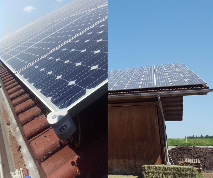
166 J. Barry et al.: Dynamic model of photovoltaic module temperature
error of 10 % in the modelled efficiency and resulting power ten in matrix notation as
output. 6
Gtot,PV
In order to describe the module temperature dynamically
T module = Mτ T amb +
one needs to solve the differential equation governing heat u1 + u2 v wind
exchange between the module and its environment, which
has been studied in detail before. Some examples include + u3 T sky − T amb , (2)
Fuentes (1987), where an approximate analytical solution is
proposed, and Jones and Underwood (2001), who show that
where the empirical coeffient u1 in units of W m−2 K−1 con-
the steady-state approach is not appropriate for 1 min time
trols the shortwave heating, u2 in W s m−3 K−1 determines
intervals. Other works in this regard are Notton et al. (2005)
the degree of convective cooling and the dimensionless pa-
and Torres Lobera and Valkealahti (2013). In Torres-Lobera
rameter u3 controls the effect of longwave thermal emission.
and Valkealahti (2014) and Gu et al. (2019) a dynamic ther-
The ambient temperature (T amb ), plane-of-array irradiance
mal model is coupled to an electrical model in order to exam- 6
ine the effect on PV module performance as a whole. In all (Gtot,PV ), wind speed (v wind ) and sky temperature (T sky ) are
cases this approach involves iteratively solving a differential time series vectors and the matrix Mτ is defined by
equation with several parameters.
In the present work a simple model built on the works of 0 for i − j < 0
exp(−(i−j )1t/τ )
Faiman (2008) and Del Cueto (2000) is modified by applying Mτ,ij = C for 0 ≤ i − j ≤ N , (3)
0 for i − j > N
an exponential smoothing kernel to represent the relaxation
time constant, which effectively includes the heat capacity of
where τ is the characteristic time constant, 1t ≡ tn − tn−1 is
the system using a matrix that introduces time dependence
the time interval between data points and the normalisation
into the equation. The four model parameters are then ex-
factor is given by
tracted from data from two measurement campaigns carried
out in autumn 2018 and summer 2019 in the Allgäu region i
X
in Germany, as part of the BMWi-funded project MetPVNet. C≡ exp (−(i − j )1t/τ ) . (4)
The model was tested and validated on two free-standing sys- j =max(0,i−N )
tems and one roof-mounted system, respectively.
The model equations are described in detail in Sect. 2. Sec- In other words, Mτ is a lower triangular matrix with e0 = 1
tion 3 outlines the measurements and data collection meth- on the diagonal and the off-diagonal entries along each row
ods, and the results and conclusions are given in Sects. 4 and are exponential functions decaying with the distance i − j
5, respectively. from the diagonal, cut off at i − j = N − 1 and normalised
by the sum of each row. Multiplying out the matrix terms
and assuming for brevity that there are at least N time steps
measured before the time point tn , one gets
2 Dynamic temperature model
N
1 X
Tmodule (tn ) = 0 exp (−k1t/τ ) Tamb (tn−k )
From physical considerations the module temperature can be C k=0
described by the heat balance equation 6
Gtot,PV (tn−k )
+ + u3 1Ts,a (tn−k ) , (5)
QSW rad − Qconv − Qnet LW rad − QPV − Qcond = 0, (1) u1 + u2 vwind (tn−k )
where 1Ts,a ≡ Tsky − Tamb and in this case the normalisa-
with the terms decreasing in approximate order of impor- tion constant C 0 is the same for each row of the matrix (in
tance: the module is heated by shortwave solar radiation and reality the normalisation is only constant after N time steps
cooled primarily by convection and longwave thermal emis- have passed). This shows that the value of module tempera-
sion, with the energy losses due to the photovoltaic effect ture from each time tn−k in the past contributes to the current
QPV (corrected for resistive losses) and conduction Qcond value at time tn , with an exponentially decreasing weight
playing a minor role (see Gu et al., 2019 for an estimation proportional to k1t/τ , up to a time 1tN. In practice one
of the importance of each term). Writing this out explicitly can simply cut off the exponential function at a small value,
leads to a differential equation with the module temperature which was chosen to be 10−6 in this work.
on both sides (see Eq. A1 in the Appendix), since the cool- Although one would expect the effect of thermal emission
4 , by factorising the corresponding
to be proportional to Tsky
ing due to convection and thermal emission depends on the
module temperature itself. term in the differential equation one can show that it is suf-
In this work a simplified parametric model is proposed as ficient to approximate the thermal emission by a term linear
follows: the module temperature time series T module is writ- in the sky temperature (see Appendix A).
Adv. Sci. Res., 17, 165–173, 2020 https://doi.org/10.5194/asr-17-165-2020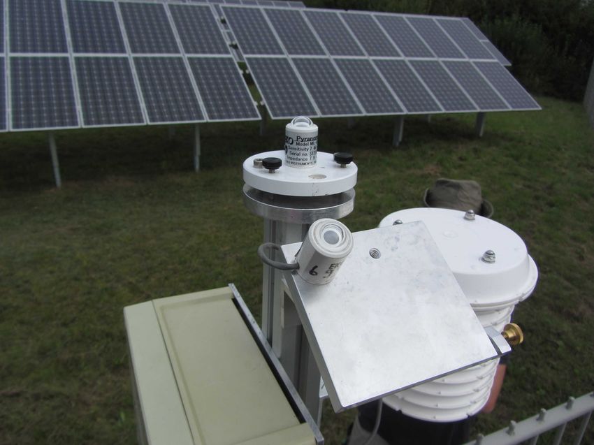
J. Barry et al.: Dynamic model of photovoltaic module temperature 167
Figure 1. PV system and measurement station with horizonal and
plane-of-array pyranometer along with a small weather station mea-
suring ambient temperature at station 1, situated at 47.683233◦ N,
10.319028◦ E.
The model in Eq. (2) has four unknown parameters: the
coefficients u1 , u2 and u3 as well as the time constant τ ,
which depend both on the characteristics of each individ-
ual PV system (i.e. its geometry, material properties or the
way it is mounted) as well as on the prevailing meteoro-
logical conditions of its surroundings. In order to be able to
apply the model to any system it is useful to perform a pa-
rameter estimation procedure using experimental data. This
so-called “forward model calibration” is performed using
non-linear inversion (Rodgers, 2000) with the Levenberg-
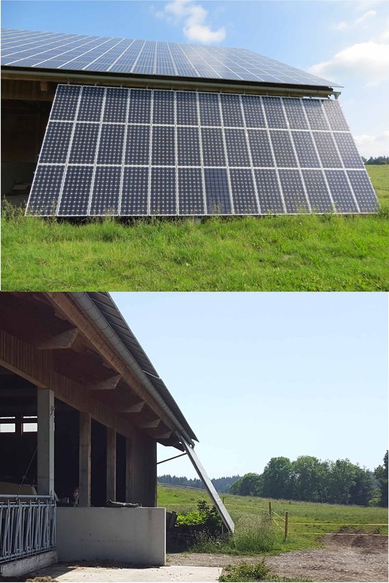
Figure 2. PV system 2A at station 2 (47.653161◦ N, 10.496584◦ E),
Marquardt method. The parameter values that give the best where the smaller system that reaches from the roof to the ground
fit between the model and the data can then be used to model was used for temperature modelling.
the module temperature at an arbitrary time point.
mounted system on top of a barn (see Fig. 3). In both cases
3 Field measurements
a temperature sensor was mounted behind the PV modules.
A pyranometer station identical to that in Fig. 1 measured ir-
3.1 Photovoltaic systems
radiance in the plane of the array of system 2A, whereas for
The model was validated using data from two different sta- system 2B a Kipp & Zonen RT1 sensor was used for this pur-
tions and three different PV systems. The first station is a pose, and an anemometer on a 5 m mast was erected closeby.
large free-standing solar park made up of 504 modules of Table 1 summarises the different quantities measured dur-
180 Wp each. The solar park is just outside Kempten, Allgäu, ing the two measurement campaigns, with their respective
close to the Iller river, and a pyranometer measuring station frequencies and uncertainties. For the temperature modelling
(see Fig. 1) as well as an anemometer on a 3 m mast were all data was downsampled to a period of 1 min using a mov-
erected on site. PV module temperature (at the back of two ing average function.
PV modules) was recorded in 15 s intervals, wind speed in
20 s intervals and irradiance and ambient temperature (mea- 3.2 Longwave atmospheric emission
sured at the pyranometer station) in 1 s intervals.
At the second station on a farm east of Kempten, two The longwave downward welling irradiance was measured
different PV systems were used to validate the model. Sys- with a frequency of 2 Hz and an uncertainty of 2 % using a
tem 2A is a small system (roughly 6 kWp) with a steep eleva- secondary standard Kipp & Zonen pyrgeometer, situated on
tion angle of roughly 60◦ and is well ventilated from behind the roof of a high-rise building in Kempten. Although this
as can be seen in Fig. 2, whereas System 2B is a larger roof- device is not exactly co-located with the PV systems it still
https://doi.org/10.5194/asr-17-165-2020 Adv. Sci. Res., 17, 165–173, 2020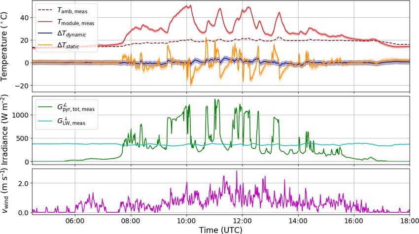
168                                                          J. Barry et al.: Dynamic model of photovoltaic module temperature

Table 1. Data frequency, measurement uncertainty and measurement time periods for the three PV systems.

                                                                                                6
                                                   Tmodule              Tamb                 Gtot                         vwind
       Station   Time period
                                              f (Hz)    σTmodule    f (Hz)   σTamb    f (Hz)        σ 6         f (Hz)        σvwind
                                                                                                     Gtot

       1         September– October 2018        1/15    ±1 K            1    ±1 K           1       ±5 %         1/20         ±0.15 m s−1
       2A        September– October 2018        1/15    ±1 K            1    ±1 K           1       ±5 %         1/20         ±0.15 m s−1
       2B        July– August 2019                 1    ±1 K            1    ±1 K           1       ±3 %          1/2         ±0.15 m s−1

                                                                      Table 2. Number of days of each type and total number of data
                                                                      points used for the parameter retrieval for each system.

                                                                        System    Time of year        Clear       Cloudy        Total data points
                                                                                                      days          days           (SZA ≤ 95◦ )
                                                                        1         Autumn 2018               6            16               11 880
                                                                        2A        Autumn 2018               8            14               16 694
                                                                        2B        Summer 2019               2             8                8895

Figure 3. PV system 2B at station 2, with a Kipp & Zonen RT1 sen-
sor mounted on the edge of the module in order to measure plane-
of-array irradiance and module temperature.

gives a general idea of the sky temperature and improves the
model fit, especially in the early morning and late evening.
The sky temperature is simply calculated from the irradiance
measurements using
        s
            ↓                                                         Figure 4. Histogram of the deviation between modelled and mea-
         4 G
            LW                                                        sured module temperature at system 1, for both the dynamic and
T sky =         ,                                        (6)
           σ                                                         static models and under all-sky conditions (i.e., all available days).
with an emissivity of  = 1 and σ the Stefan-Boltzmann con-
stant. Any deviations from blackbody emissions as well as a
reduction in the field of view due to the tilt of the PV mod-         with the parameters u1,2,3 allowed to vary but with τ = 0.
ules will be captured in the variation of the coefficient u3 in       The number of days of each type are shown in Table 2, as
Eq. (2).                                                              well as the time of year in which the measurements were
                                                                      taken. The multiparameter fit was performed for all days at
                                                                      once: the third column of Table 2 gives the total number of
4   Results                                                           data points for each system, i.e., the length of the time series
                                                                      vectors in Eq. (2) in 1 min resolution. Note that only data up
The model in Eq. (2) (referred to as the “dynamic” model)
                                                                      to a solar zenith angle (SZA) of 95◦ were considered.
was fitted to the module temperature for the three systems
described above, for different days during the measurement
campaigns in 2018 and 2019. To illustrate the effect of
adding time-dependence to the model, another fit with the
so-called “static” or time-independent model was performed,

Adv. Sci. Res., 17, 165–173, 2020                                                          https://doi.org/10.5194/asr-17-165-2020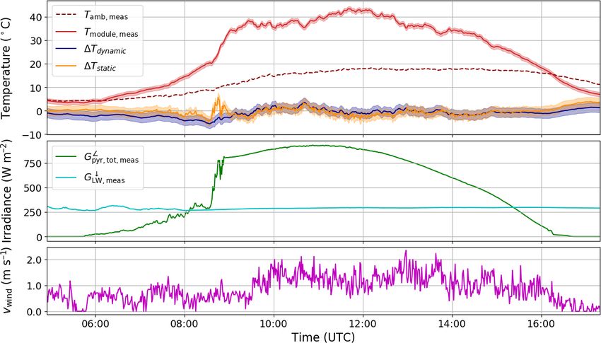
J. Barry et al.: Dynamic model of photovoltaic module temperature                                                                     169

Table 3. Results for all-sky conditions for both the static and dynamic models.

                                      System 1                             System 2A                            System 2B
   Parameter
                                Dynamic               Static          Dynamic               Static         Dynamic               Static
   u1 (W m−2 K−1 )        26.774 ± 0.051    35.045 ± 0.063     27.182 ± 0.043     32.699 ± 0.048      31.157 ± 0.119   37.360 ± 0.110
   u2 (W s m−3 K−1 )       4.355 ± 0.034     2.958 ± 0.038      4.155 ± 0.018      3.517 ± 0.019       3.653 ± 0.042    2.782 ± 0.038
   u3                      0.207 ± 0.001     0.038 ± 0.001      0.010 ± 0.001     −0.083 ± 0.001       0.158 ± 0.002    0.063 ± 0.002
   τ (s)                     588.8 ± 2.9                 –        508.9 ± 2.5                  –         547.4 ± 5.2                –
   RMSE (K)                          1.35              3.31               1.20               2.67               2.18              3.11
   |1T |max (K)                      5.83             21.84               6.28              18.96               7.63             19.27

Figure 5. Comparison of dynamic and static temperature modelling for system 1 on 14 September 2018. Measured module temperature
(red) is plotted together with the deviation between modelled and measured module temperature for the dynamic (blue) and static (orange)
models, along with ambient temperature (dark red dashed), in units of ◦ C. Shortwave (green) and longwave (cyan) irradiance as well as wind
speed (magenta) are also shown.

   The a priori values of the unknown parameters were taken             der to correctly model the instantaneous temperature of PV
to be                                                                   modules one has to consider a dynamic approach.
                                                                           Figure 5 shows the model results for system 1 on
u1,a = 25 W m−2 K−1 ,       u2,a = 7 W s m−3 K−1 ,                      14 September 2018, a day with high variability in global ra-
u3,a = 0.25,    and τa = 600 s,                                 (7)     diation. The measured temperature with its uncertainty can
                                                                        be compared to the modelled temperature using both mod-
with an a priori uncertainty of 20 % for the parameters ui,a            els, and the corresponding ambient temperature, irradiance
(i = 1, 2, 3) and 50 % for τa . The results of both modelling           and wind speed are plotted for completeness. The dynamic
approaches are compared in Table 3, for all-sky conditions              model can reproduce the measured module temperature, even
(i.e., all available days). It is evident that the dynamic model        during times with fluctuating irradiance. The time constant is
shows a better fit to the data: the RMSE is roughly halved              found to be of the order of 10 min (see Table 3), which can
from 3.03 to 1.58 K, on average. An even larger reduction               also be seen by examining the typical width of the troughs
can be seen in the maximum absolute deviation |1T |max :                and peaks in the temperature curve during cloudy conditions.
the static model has a maximum absolute deviation ranging               In addition, after sunset the module temperature falls below
from 18.96 to 21.84 K, with a mean of 20.02 K, whereas the              ambient temperature and the inclusion of longwave thermal
dynamic model gives a range of 5.83 K ≤ |1T |max ≤ 7.63 K               emission in the model allows the temperature at this time of
and a mean of 6.58 K. The histogram in Fig. 4 shows that                day to be modelled accurately.
the error in the static model for system 1 has a much larger
spread than that of the dynamic model. This shows that in or-

https://doi.org/10.5194/asr-17-165-2020                                                              Adv. Sci. Res., 17, 165–173, 2020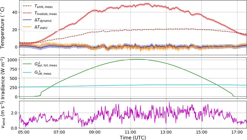
170                                                          J. Barry et al.: Dynamic model of photovoltaic module temperature

Figure 6. Comparison of dynamic and static temperature modelling for system 2A on 27 September 2018, see the caption of Fig. 5 for
details.

Figure 7. Comparison of dynamic and static temperature modelling for system 1 on 4 October 2018, see the caption of Fig. 5 for details.

   The model can also reproduce the thermal behaviour on               camera next to the system confirmed the presence of fog, and
a clear sky day, as shown in Fig. 6. In this case the static           since the module temperature is higher than predicted it is
model reproduces the high frequency variations in temper-              most probably due to an incorrect sky temperature, since the
ature due to the varying wind speed, whereas the dynamic               measurement of thermal emission is situated north of the PV
model smooths them out (the exponential term acts like a               system on a high-rise building with different overhead con-
lowpass filter). Note that the non-linear fitting procedure was        ditions.
applied to all data at once (both clear and cloudy days), so
that the algorithm finds the optimal parameters that will min-         5   Conclusions
imise the cost function over the entire time series (see Ta-
ble 2). One case in which the model shows a larger deviation           In this work a simple four-parameter dynamic thermal model
from measurement is in the presence of low-lying fog, as can           for the temperature of PV systems was proposed, and the
be seen in Fig. 7, for system 1 on 4 October 2018. A cloud             model was fitted to data from three different systems us-

Adv. Sci. Res., 17, 165–173, 2020                                                           https://doi.org/10.5194/asr-17-165-2020
J. Barry et al.: Dynamic model of photovoltaic module temperature                                171

ing non-linear optimisation. By employing an exponential
smoothing kernel it was shown that the time constant (and
therefore the heat capacity) of the system can be extracted
from data, and the dynamic model could reproduce 1 min
instantaneous temperature measurements with an RMSE of
between 1.20 and 2.18 K and a maximum absolute deviation
of between 5.83 and 7.63 K. Further improvements to this
work could be achieved by considering reflection losses as
well as losses due to power generation. It could also be con-
ceivable to use the measured PV power to estimate the sky
temperature, so that a longwave irradiance measurement is
not needed. A comprehensive comparison of the differential
equation approach with the method presented here will be
carried out in future work.

https://doi.org/10.5194/asr-17-165-2020                             Adv. Sci. Res., 17, 165–173, 2020
172                                                          J. Barry et al.: Dynamic model of photovoltaic module temperature

Appendix A: Physically motivated approach                               Assuming that glass = tedlar ≡ , the thermal emission
                                                                     term in Eq. (A1) can be rewritten as
From the heat balance equation in Eq. (1) and ignoring con-                                  h
duction one can write down the differential equation for the               4          4              2         2
                                                                      σ (Tmodule − Tsky ) =  σ Tmodule   + Tsky
thermal exchange between a free-standing PV module with
                                                                                                          i
inclination angle θ and its environment as                                                 Tmodule + Tsky    Tmodule − Tsky

Cmodule dTmodule      ↓    6                                                               ≡ hrad,s Tmodule − Tsky ,          (A2)
                  = αPV Gtot,PV − hconv
  A        dt
                                                                     and it turns out that the term hrad,s is roughly constant. A
        (Tmodule − Tamb )
                                                                   similar term hrad,g can be written for the term dependent
                    1 + cos θ            1 − cos θ                   on Tground , for which the same conclusion applies. This ap-
        − σ glass             + tedlar
                        2                     2                      proach is used in Fuentes (1987) in order to calculate an ap-

           4
          Tmodule     4
                  − Tsky                                             proximate analytical solution to Eq. (A1), and in this way the
                                                                   simple parametric models can be shown to be approximately
                    1 − cos θ            1 + cos θ                   equivalent to the physically motivated approach. A compre-
        − σ glass             + tedlar
                        2                     2                      hensive comparison will be carried out in future work.
                                          6
           4          4
          Tmodule − Tground − ηmodule Gtot,PV ,             (A1)

where ηmodule is the electrical efficiency, Cmodule is the
heat capacity in J K−1 , hconv is the convective coefficient in
               ↓
W K−1 m−2 , αPV is the absorptivity for shortwave radiation
at normal incidence, glass (tedlar ) is the emissivity for long-
wave radiation from the glass (tedlar) surface and σ is the
Stefan-Boltzmann constant.

Adv. Sci. Res., 17, 165–173, 2020                                                       https://doi.org/10.5194/asr-17-165-2020
J. Barry et al.: Dynamic model of photovoltaic module temperature 173
Data availability. Data is available as an open-access data set via Del Cueto, J. A.: Model for the thermal characteristics of flat-plate
https://doi.org/10.5281/zenodo.3958820 (Barry et al., 2020). photovoltaic modules deployed at fixed tilt, Conference Record
of the Twenty-Eighth IEEE Photovoltaic Specialists Conference
– 2000, 15–22 September 2000, Anchorage, AK, USA, 1441–
Author contributions. The two measurement campaigns were 1445, https://doi.org/10.1109/PVSC.2000.916164, 2000.
designed and coordinated with contributions from all authors, and Faiman, D.: Assessing the Outdoor Operating Temperature
the installation and calibration of the various measurement devices of Photovoltaic Modules, Prog. Photovoltaics, 16, 307–315,
was performed by NK, CS, HD, JW and FG. The temperature model https://doi.org/10.1002/pip.813, 2008.
was developed by JB, DB, KP, AHC and SM; the software and sim- Fuentes, M. K.: A Simplified Thermal Model for Flat-Plate
ulations to implement the model were developed and carried out by Photovoltaic Arrays, Tech. rep., Sandia National Labs, Albu-
JB and DB. JB prepared the manuscript with contributions from all querque, NM, USA, available at: https://prod-ng.sandia.gov/
co-authors. techlib-noauth/access-control.cgi/1985/850330.pdf (last access:
24 July 2020), 1987.
Gu, W., Ma, T., Shen, L., Li, M., Zhang, Y., and Zhang,
Competing interests. The authors declare that they have no con- W.: Coupled electrical-thermal modelling of photovoltaic
flict of interest. modules under dynamic conditions, Energy, 188, 116043,
https://doi.org/10.1016/j.energy.2019.116043, 2019.
Jones, A. D. and Underwood, C. P.: A thermal model
for photovoltaic systems, Sol. Energy, 70, 349–359,
Special issue statement. This article is part of the special issue
https://doi.org/10.1016/S0038-092X(00)00149-3, 2001.
“19th EMS Annual Meeting: European Conference for Applied Me-
King, D. L., Boyson, W. E., and Kratochvil, J. A.: Photovoltaic ar-
teorology and Climatology 2019”. It is a result of the EMS Annual
ray performance model, Tech. Rep. December, Sandia National
Meeting: European Conference for Applied Meteorology and Cli-
Laboratories, https://doi.org/10.2172/919131, 2004.
matology 2019, Lyngby, Denmark, 9–13 September 2019.
Notton, G., Cristofari, C., Mattei, M., and Poggi, P.: Mod-
elling of a double-glass photovoltaic module using fi-
nite differences, Appl. Therm. Eng., 25, 2854–2877,
Acknowledgements. This research was carried out under https://doi.org/10.1016/j.applthermaleng.2005.02.008, 2005.
the BMWi project “MetPVNet: Entwicklung innovativer satel- Rodgers, C. D.: Inverse Methods for Atmospheric Sounding: The-
litengestützter Methoden zur verbesserten PVErtragsvorhersage auf ory and Practice, WorldScientific, Oxford, UK, 2000.
verschiedenen Zeitskalen für Anwendungen auf Verteilnetzebene”. Skoplaki, E. and Palyvos, J.: On the temperature dependence
Thanks go to Philipp Hofbauer and Matthias Struck from egrid ap- of photovoltaic module electrical performance: A review
plications & consulting GmbH (part of the local grid operator All- of efficiency/power correlations, Sol. Energy, 83, 614–624,
gäuer Überlandwerk), for access to the photovoltaic systems in the https://doi.org/10.1016/J.SOLENER.2008.10.008, 2009a.
Allgäu region. Skoplaki, E. and Palyvos, J. A.: Operating temperature of pho-
tovoltaic modules: A survey of pertinent correlations, Renew.
Energ., 34, 23–29, https://doi.org/10.1016/j.renene.2008.04.009,
Financial support. This research has been supported by the Bun- 2009b.
desministerium für Wirtschaft und Energie (grant no. 0350009). Torres Lobera, D. and Valkealahti, S.: Dynamic thermal model of
solar PV systems under varying climatic conditions, Sol. Energy,
93, 183–194, https://doi.org/10.1016/j.solener.2013.03.028,
Review statement. This paper was edited by Sven-Erik Gryning 2013.
and reviewed by David Faiman and one anonymous referee. Torres-Lobera, D. and Valkealahti, S.: Inclusive dynamic ther-
mal and electric simulation model of solar PV systems un-
der varying atmospheric conditions, Sol. Energy, 105, 632–647,
https://doi.org/10.1016/j.solener.2014.04.018, 2014.
References
Barry, J., Böttcher, D., Pfeilsticker, K., Herman-Czezuch, A., Kimi-
aie, N., Meilinger, S., Schirrmeister, C., Deneke, H., Witthuhn, J.,
and Gödde, F.: Supplement to “Dynamic model of photovoltaic
module temperature as a function of atmospheric conditions”
(Version 1), Zenodo, https://doi.org/10.5281/zenodo.3958820,
2020.
https://doi.org/10.5194/asr-17-165-2020 Adv. Sci. Res., 17, 165–173, 2020You can also read


