On the Influence of Weather Forecast Errors in Short-Term Load Forecasting Models - NUI Galway
←
→
Page content transcription
If your browser does not render page correctly, please read the page content below
1
On the Influence of Weather Forecast Errors in
Short-Term Load Forecasting Models.
D. Fay and J.V. Ringwood
to use weather information for future load forecasts, weather
Abstract-- Weather information is an important factor in load forecasts must be utilised and these have associated weather
forecasting models. Typically, load forecasting models are forecast errors. Although system dependent, weather forecast
constructed and tested using actual weather readings. However, errors can be significant [5] and have been attributed as the
online operation of load forecasting models requires the use of
cause of 17% [6] to 60% [7] of load forecast errors.
weather forecasts, with associated weather forecast errors. These
weather forecast errors inevitably lead to a degradation in model Load forecasting models are usually trained using actual
performance. This is an important factor in load forecasting but past weather readings as opposed to past weather forecasts [8].
has been widely examined in the literature. The main aim of this This is based on the assumption that to use the latter
paper is to present a novel technique for minimizing this essentially adds forecast noise to the training data. Often
degradation. In addition, a supplementary technique is proposed weather forecasts are unavailable for the entire training period
to model weather forecast errors to reflect current accuracy.
and/or can be subject to increasing accuracy of meteorological
The proposed technique combines the forecasts of several load
forecasting models. This approach allows the parameters of the models, as mathematical weather models are constantly
load forecasting models to be estimated using actual weather, thus improved. Therefore, training load models with actual weather
avoiding introducing noise (i.e. weather forecast error) into the can be justified [8]. However, when weather forecast errors
training input set. The effect of the weather forecast error is then not present in the training set are presented, they can have a
minimised during the combination stage. disproportionate influence on load models [9]. Changing the
load model parameters to account for this can be impossible in
Index Terms-- Load forecasting, weather forecast errors,
many conventional models once training is completed.
model combination, data fusion.
Douglas et al. [6] approached this problem by use of a
I. INTRODUCTION Bayesian framework, but restricted analysis to the use of
dynamic linear models. In spite of the importance of weather
S hort Term Load Forecasting (STLF) refers to forecasts of
electricity demand (or load), on an hourly basis, from one
to several days ahead. The amount of excess electricity
forecast errors with respect to load forecasting, the literature is
sparse [10,11].
This paper proposes combining several models (called sub-
production (or spinning reserve) required to guarantee supply,
models), or model fusion, as a technique for minimising the
in the event of an underestimation, is determined by the
effect of weather forecast errors in load forecasting models.
accuracy of these forecasts. Conversely, overestimation of the
The concept of model fusion is well known in the general field
load leads to sub-optimal scheduling (in terms of production
of forecasting and was pioneered mainly in [12]. Fused
costs) of power plants (known as unit commitment). In
forecasts are theoretically more accurate than any of the
addition, a deregulated market structure exists in Ireland which
individual model forecasts [13,14] as different models are
in which load forecasts play a central role.
often better at modelling different aspects of an underlying
As illustrated above, STLF is an important area and this is
process and thus combining the models appropriately gives a
reflected in the literature by the many techniques that have
better forecast. In addition, a single model incorporating all
been applied, including neural networks [Hippert 1], fuzzy
aspects of an underlying process may be more complex and
logic [Mastorocostas 2] and statistical techniques [H. Chen 3],
difficult to train than combining individual models [13].
to mention but a few. In many electricity grid systems, the
However, it should be noted that a fusion model is not a
prevailing weather has a significant effect on the load and it
universal approximator as information may be lost by the sub-
has been found that including weather information can
models which cannot be recovered by the fusion model. Model
improve a load forecast [tamimi 4, chen3]. However, in order
fusion is particularly suited to STLF as the sub-models may be
trained with actual weather information and the effect of
The authors wish to thank Eirgrid, the Irish national grid operator, for weather forecast errors taken into account when combining the
their assistance in this research.
Dr. Damien Fay is with the department of Mathematics, NUI, Galway, models.
Ireland, (Damien.fay@nuigalway.ie). Professor John Ringwood is with the
department of Electronic Engineering, NUI, Maynooth, Ireland.
(john.ringwood@eeng.nuim.ie).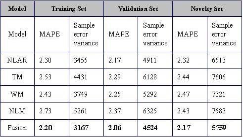
2
II. DATA SET DETAILS and climate change [15]. Previous approaches in STLF have
The range and time-scale of the available electrical demand modelled the weather forecast error simply as a Gaussian
data is given in Table 1. random variable [16, 17]. However, as seen in Figure 1 this is
TABLE I not an accurate representation of the statistics of the weather
DATA TIME-SCALE AND RANGE forecast errors in Ireland. Rather, the forecast error displays
serial correlation, i.e. it is either above or below the actual for
prolonged periods. Typically some form of aggregate weather
variables are normally used in STLF models (e.g. average
daily temperature). The error in an aggregate weather variable
will have a non-zero mean (Figure 1) and a Gaussian
approximation would underestimate this.
The weather in Ireland is dominated by Atlantic weather
Two categories of historical weather data are available from systems. When a weather system or front reaches Ireland there
the Meteorological Office of Ireland (MOI): readings (or is a shift in the level of the temperature and other weather
actual weather) and forecasts. Both sets of data are for Dublin variables (Figure 1) (a similar situation is noted in [3]). This
airport, the closest and most relevant weather station to Dublin shift is also a factor that the Irish Meteorological Office must
(Table 2). The readings and forecasts are for dry bulb forecast. The weather forecast error is thus assumed to have
temperature, cloud cover, wind speed and wind direction. the following structure:
TABLE II • Turning points (Figure 1) which represent the arrival of a
WEATHER DATA TIME-SCALE AND RANGE
weather front,
~
• A level error, µ , which is the average of the weather
forecast error between turning points,
• A shape error, σ~ , which is the standard deviation of the
weather forecast error between turning points, and
• A random error, which accounts for the remaining error if
µ~ and σ~ are removed.
The data is subdivided into three sets in order to train and
test the load forecasting models (Table 3). The training set is
used to calculate model parameters, the validation set is used
to aid in model structure determination and the novelty set is
used to evaluate model performance.
TABLE III
DIVISION OF DATA SET
Data between Monday and Friday in the months January to
March (known as the “late winter working day day-type”) is
selected so as to avoid the exceptions associated with Fig. 1. Actual and forecast temperature (6th to 15th February 2000).
weekend, Christmas and changes due to the daylight saving
hour. In order to detect the turning points the following algorithm
was found to be sufficient. The weather variable is first
III. MODELING WEATHER FORECAST ERRORS. smoothed by means of a state space model based on an
Due to the sparseness of weather forecast data (Table 2) it integrated random walk:
is necessary to model the weather forecast error to produce 1 1
pseudo-weather forecasts for the entire data set. Indeed, even
X (k ) = X (k − 1) + ε (k ) (1)
0 1
given a long database of weather forecasts, this may be a good
where X(k) is the state vector at time k and ε(k) is the process
idea. This is because the quality of weather forecasts is
noise. The temperature is then extracted from the state vector
changing over time due to improved forecasting techniques3
by means of the measurement equation: the pseudo-temperature forecast errors. As can be seen, the
y (k ) = [1 0] X (k ) + ν (k ) (2) SACF for both are similar, showing that the pseudo-forecast
errors have captured the auto-correlation evident in the
where y(k) is the filtered weather variable and ν (k ) is the
temperature forecast errors. A similar situation was found with
measurement noise. The state vector is estimated using the
the other weather variables.
Kalman filter (Note: the a- posteriori state vector estimate is
used in (2) as a smoothed version of the original is desired
[18]). The turning points are then defined as the maxima and
minima within a rolling window of length 5:
11 y ( k − 5 + i )
y = y (k ) / y (k ) .5 ∑ , i ≠ 5, ∀k (3)
i =0 10
where y is the set of turning points and denotes greater or
less than. A sample of the turning points detected by this
algorithm are shown in fig. 2, below.
Fig. 4. SACF of forecast and pseudo-forecast temperature errors.
Fig. 2. A sample of the turning points calculated for temperature.
IV. THE FUSION MODEL
Fig. 3 below shows the histograms, fitted Gaussian
A. Preliminary Auto-Regressive (AR) linear model.
distributions and the Sample AutoCorrelation Function
(SACF) for the level shape and random error of the It was previously found by these authors [19] that
temperature forecasts. decomposing load data into 24 parallel series, one for each
hour of the day, is advantageous as the parallel series have a
degree of independence. The parallel series for hour j on day
k, y(j,k), has a low frequency trend, d(j,k), which is first
removed using a Basic Structural Model (BSM) leaving a
residual, x(j,k), (Figure 5) which is composed of weather, non-
linear auto-regressive and white noise components [19].
Fig. 5. Preliminary AR linear model overview.
B. Sub-Models.
Fig. 3. Distributions and SACF for temperature forecasts.
Three models were chosen which have different types of
The shape and level errors of the four weather variables are inputs. These are chosen so that forecast errors can be
found to be cross correlated, suggesting that they may be attributed to particular inputs. A fourth model is included
jointly distributed. In order to generate pseudo-weather using all the available inputs to capture any non-linear
forecast errors, the turning points in the actual weather relationships between the inputs and the residual. The models
variables are first identified. Then, a multivariate Gaussian are named after their input types as shown in fig. 4. The fusion
pseudo-random number generator is used to generate the technique combines the forecasts of the sub-models,
random errors for each the weather variables jointly. Fig. 4, xˆ1 ( j , k ),..., xˆ 4 ( j , k ) , to give a fused forecast, xˆ f ( j , k ) of the
below, shows the SACF of the temperature forecast errors and residual for series j on day k (Fig. 6).4
It was found that this improved the prediction performance of
the models in all cases.
The Temperature Model (TM) input, t(j,k), is a vector of
the previous 72 hours of temperature from hour j on day k.
Similarly the other Weather Model (WM) uses vectors of wind
speed, w(j,k), cloud cover, c(j,k), and wind direction, q(j,k) for
the previous 72 hours of weather. The Non-Linear Auto-
Regressive model (NLAR) uses the previous 2 days of
residual, x(j,k-1) and x(j,k-2). The Non-Linear Model (NLM)
uses all the available inputs.
C. Fusion Algorithm.
The data fusion algorithm described in [21] seeks to
minimize the variance of the fused forecast based on the
covariance matrix of the sub-model forecasts. The cross-
covariance of the forecasts is considered and the distribution
of the forecast error noise is not restricted to Gaussian but
merely required to be unbiased. A combined forecast, xf(j,k),
of the load is created using a weighted average of the
Fig. 6. Data fusion model overview. individual forecasts xˆ1 ( j , k ),..., xˆ 4 ( j , k ) [21]:
4
The sub-models all use feed forward neural networks, x f ( j , k ) = ∑ Ai ( j ) xi ( j , k ) (5)
although it should be noted that the choice of modelling i =1
technique is not central to this paper. Initially, the traditional where Ai(j) is the weight applied to the forecast from sub-
back-propagation algorithm using Levenberg-Marquadt with model i for hour j2, and is derived from the error covariance
cross validation was used to train the networks. Each of the matrices of xˆ1 ( j , k ),..., xˆ 4 ( j , k ) as:
networks has two hidden layers and a single output. To
determine a suitable structure for the network (i.e. the number
of nodes in each layer), different network structures were [ A1 ( j ) A2 ( j ) A3 ( j )] = [ P4' ,1 ( j ) P4' ,2 ( j ) P4' ,3 ( j )]P −1 (6)
trained (ranging from a 1×1 to a 7×7 network) and their
Prediction Mean Squared Errors (PMSE) compared over the where P4',1 ( j ) , P4', 2 ( j ) , P4',3 ( j ) and P are auxiliary variables
validation set. The best structure was then selected for further
derived from the sample error covariance of
evaluation.
xˆ1 ( j , k ),..., xˆ 4 ( j , k ) :
Given these initial models, the residuals where then
examined for homogeneity of variance and it was concluded 1 M
Pi ,n ( j ) =∑ ( x( j , k ) - xˆ i ( j , k ))( x( j , k ) - xˆ n ( j , k )) (7)
that the time series possessed non-constant variance. The most M k =1
likely cause for the non-constant variance lies in the where Pi,n(j) is the error covariance of sub-model i with sub-
considerable growth experienced in Irish electricity demand model n for hour j, and M is the number of samples used. The
auxiliary variables are then defined as:
over the period of the data set. With the increase in electricity
demand a corresponding increase in forecasting error (and thus P4' ,i ( j ) = P4,4 ( j ) − P4,i ( j ) i≠4 (8)
variance) would be expected. The standard approach in this and
case is to presume that the variance is proportional to the level P1',1 ( j ) P1',2 ( j ) P1',3 ( j )
of the time series squared, specifically y 2 ( j , k ) , and then to
P = P2' ,1 ( j ) P2' ,2 ( j ) P2' ,3 ( j ) (9)
scale the errors using weighted least squares [20]. During '
P ( j ) P3',2 ( j ) P3',3 ( j )
training with the back-propagation algorithm the target errors 3,1
are thus scaled prior to being propagated backwards as: where
1 Pi',n ( j ) = Pi,n ( j ) − P4,n ( j ) − Pi,4 ( j ) + P4,4 ( j ) i ≠ 4, n ≠ 4 (10)
y ( j ,1) 0 0 The final weight A4 is determined using the constraint that xf(j)
0 1 is unbiased:
0
e' = y ( j ,2) e j = 1,...,24 (4) 3
A4 ( j ) = 1 − ∑ Ai ( j ) (11)
i =1
0 1
0
y ( j , N )
2
Although it is assumed that the variance is proportional to y2(j,k), an
adjustment for heteroskedasticity is not necessary here as multiplying Pin(j) by
where e is vector of target errors and e’ is the adjusted vector. a scaling factor will not change the weights.5
Finally the fused load forecast, y f ( j , k ) , is estimated by TABLE V
AN EXAMPLE OF FUSION WEIGHTS (ACTUAL WEATHER INPUTS)
reintroducing the trend:
yˆ f ( j , k ) = dˆ ( j , k ) + xˆ f ( j , k ) (12)
V. RESULTS.
The overall approach suggested here is that the sub-model
parameters are estimated using actual weather inputs (thus Fig. 7 below shows the Mean Absolute Percentage Error
estimating the sub-model parameters without pseudo-weather (MAPE)* for the sub-models and the fusion model in Case I.
forecast errors). The error covariance matrices of the sub- As can be seen the fusion model performs best for each hour
models (10) are then estimated using pseudo-weather of the day.
forecasts as input. The weights, Ai(j), are then estimated using
these error covariance matrices. However, the results are here
analysed for two cases. The first examines the behaviour of the
fusion model without pseudo-weather forecasts and the second
examines the behaviour with them:
Case I: The sub-model parameters are estimated using actual
weather inputs (thus estimating the sub-model parameters
without pseudo-weather forecast errors). The error covariance
matrices of the sub-models (10) are then estimated using
actual weather inputs. The weights, Ai(j), are then calculated
using these error covariance matrices (as in Section IV part C).
Case II: The sub-model parameters are estimated using actual
weather inputs (as in case I). The error covariance matrices of
the sub-models (10) are then estimated using pseudo-weather
forecast inputs (unlike Case I). The weights, Ai(j), are then Fig. 7. MAPE as a function of hour of the day for fusion and sub-models
calculated using these (new) error covariance matrices (as in (notes: novelty set, actual weather used).
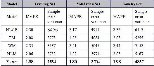
Section IV part C). Models are trained and evaluated using
Table VI below, summarise's the results in the training,
pseudo weather forecast inputs.
validation and novelty data sets.
As an example, the cross-covariance matrix of sub-model
TABLE VI
forecast errors is shown in Table IV below for the midday MODEL PERFORMANCE USING ACTUAL WEATHER INPUTS.
series (j=12). The difference between case I and II is indicated
by an arrow. As can be seen the covariance of sub-models 2 to
4 increases when pseudo-weather forecasts are used. This
increase indicates the degradation of the models due to
(pseudo) weather forecast error.
TABLE IV
THE CROSS-COVARIANCE MATRIX OF SUB-MODEL LOAD FORECAST ERRORS (CASE I→
CASE II)
Fig. 8 below shows the Mean Absolute Percentage Error
(MAPE) for the sub-models and the fusion model using
pseudo-forecast weather inputs in the novelty set. The effect of
weather forecast errors are now accounted for by calculating
the error covariance matrices of the sub-models over the
The corresponding values of A1,…A4 are shown in Table V training set with pseudo-weather forecast inputs. As can be
below. As can be seen the weights are approximately equal seen the fusion model again performs best for each hour of the
showing that each model has similar forecast accuracy. Note day.
however, how the weights change significantly once pseudo-
weather forecasts are introduced to the models. *
The MAPE is the standard error measure in the field of STLF as it allows
comparison between systems.6
v( j ) = e1 ( j ) + e2 ( j ) (14)
where u(j) and v(j) are observations of the random variables U
and V respectively. As cov(U,V) = σ 12 − σ 22 (see [22] for more
details) and we wish to show that σ 12 − σ 22 ≠ 0 a null
hypothesis may be constructed as:
H0: cov(U,V) = 0 (15)
This may be tested [22] using the test statistic:
SUV asy.
~ N (0,1) (16)
[ ]
n u 2 ( j )v 2 ( j ) / n 2 1 / 2
∑ j =1
where SUV is the sample cross covariance between U and n is
the number of samples used.
Note that in Section IV part B it was assumed that the
variance of the errors is proportional to value of the time
series. As the test statistic in (16) is based on the assumption
of constant variance, the forecast errors (from the NLAR
Fig. 8. MAPE as a function of hour of the day for fusion and sub-models model and fusion model) are first scaled as in (4) prior to
(notes: novelty set, pseudo-weather forecasts used). constructing the test statistic in (16).
TABLE VII
Fig. 9 (panel 1) below, shows an example plot of the
SUMMARY OF THE MAPE'S OF THE MODELS USING PSEUDO WEATHER FORECAST INPUTS. forecasting errors for the NLAR model, e1(j,12), and the
fusion model, ef(j,12) (note: this is for the mid-day series,
k=12). As can be seen there is a high degree of cross-
correlation between the forecast errors. Panel 2 and 4 show the
histogram of e1(j,12) and u(j,12) which appears to show that
they are drawn from a normal distribution. Panel 3 shows a
plot of u(j,12) for completeness. The corresponding plots for
ef(j,12) and v(j,12) are similar.
Comparing Tables IV and V, it can be seen that the NLAR
models are unaffected by weather forecast errors as they have
no weather inputs. The other sub-models deteriorate with the
inclusion of pseudo-weather forecast errors. The fusion model
deteriorates with the inclusion of pseudo-weather forecast
error but maintains its position as the best model.
Next the question must be asked if the difference between
the performance of the fusion model and the other models is
actually significant or due to chance. For this purpose the
errors from the NLAR sub-model (the best sub-model) are
compared to those from the fusion model. First it should be
noted that the errors from the fusion model are correlated to
Fig. 9. Plots and histograms of the forecast errors and their differences.
those from the NLAR sub-model and so the assumptions (notes: novelty set, pseudo-weather forecasts used).
underlying the standard Theil test are violated.
In general, under the assumptions that the forecast errors of Table VIII below gives a summary for the statistics used in
two estimators, e1(j) and e2(j), are cross-correlated, zero mean ensuring that the assumptions required for (16) hold (as an
and possess constant variance, σ 12 and σ 22 resp.; a test example the mid-day time series is used). The t-test is used to
statistic may be constructed based on the difference, u(j) and check that the residuals are zero mean which is confirmed in
sum, v(j) of their errors [22]: all cases. The Ljung-Box test is used to test if the residuals are
u ( j ) = e1 ( j ) − e2 ( j ) (13) random. It was found that there does exist some serial
correlation in the residuals, however this is not evident until
and
later lags. The Jarque-Bera test is used to test for normality. It7
is found that the hypothesis of normality is rejected. On further Fig. 10. P-values for each hour of the day. (notes: novelty set, pseudo-
weather forecasts used).
examination this is due to several outliers on the right tail of
the distribution. These are caused by the large error which
VI. CONCLUSION
occurs between the transitions from year to year in the late
winter working day day-type. Given this limitation the This paper examined the effect of weather forecast errors in
hypothesis (15) is tested. load forecasting models. In Section 3, the distribution of the
weather forecast errors was examined and it was found that a
TABLE VIII Gaussian distribution was not appropriate in this case. Rather,
SUMMARY OF FORECAST ERROR STATISTICS . (k=12)
a structure exists which means that the weather forecast error
Result (0
Sample(s) Test Hypothesis Significance Power –accept, will have a large effect on any aggregate weather variables.
1-reject). The structure of the weather forecast errors was then used
H0:mean=0 to produce pseudo-weather forecast errors from 1986 to 2000
e1(j) t-test 5% 0.86 0
H1:mean≠0
which have the accuracy of current weather forecasts. This is
H0:mean=0
ef(j) t-test 5% 0.90 0 important as, for example, weather forecasts from 1986 are
H1:mean≠0
5% (lag 1) 0.4 0 less accurate than current weather forecasts and thus of no
5% … 0.6 0 relevance in predicting future loads.
Ljung-Box Series is
e1(j) 5% … 0.7 0
test random A model fusion technique was then proposed for
5% … 0.07 0
5% (lag5) 0.01 1 minimising the effect of weather forecast errors. In general
5% (lag 1) 0.72 0 weather forecast error causes approximately 1% deterioration
5% … 0.86 0 in load forecasts of all models used here. This figure, though
Ljung-Box Series is
ef(j) 5% … 0.92 0
test random important, is not as high as suggested by [6] and [7], for their
5% … 0.05 0
5% (lag5) 0.03 1 systems. However, the fusion model was capable of adjusting
e1(j) Jarque- H0: e1(j)~N 5% 0.0023 1 the weighting of the sub-models to reflect that the weather
Bera test H1: e1(j) based sub-models deteriorated relative to the AR model.
skewed
Finally, the fusion model was shown to successfully separate
e2(j) Jarque- H0: e1(j)~N 5% 0.0002 1
Bera test H1: e1(j) the tasks of model training and rejecting weather forecast
skewed errors.
e1(j), e2(j) Eqn. (15) H0: cov(U,V) 5% 0.9972 0
=0 VII. REFERENCES
[1] S.H. Hippert, C.E. Pedriera, R.C. Souza, "Neural networks for short-
Fig. 10 below, shows the p-value for the testing the term load forecasting: a review and evaluation", IEEE Transactions on
hypothesis that the variance of the residuals from the two Power Systems, 16 (1), pp. 44-55, 2001.
models are statistically different. As there are 24 hours, 24 [2] P.A. Mastorocostas, J.B. Theocharis, S.J. Kiartzis, A.G. Bakisrtzis, "A
hybrid fuzzy modeling method for short-term load forecasting",
tests are conducted. The results show that the hypothesis is Mathematics and Computers in Simulation, 51, pp. 221-232, 2000.
accepted at the 1% confidence level for most of the hours, at [3] H. Chen, Y. Du, J.N. Jiang, “Weather sensitive short-term load
the 5% confidence level for all but one of the hours where the forecasting using knowledge-based ARX models”, IEEE Power
Engineering Society General Meeting, Vol 1, pp 190-196, 12-16 June
p-value is 0.83. Thus empirical evidence would seem to show 2005.
that the fusion model is indeed a better model than the NLAR [4] M. Tamimi, R. Egbert, "Short term electric load forecasting via fuzzy
model. neural collaboration", Electric Power Systems Research, 56, pp. 243-
248, 2000.
[5] T. J., Teisberg, , R. F. Weiher, and A. Khotanzad, “The value of national
weather service forecasts in scheduling electricity generation.”, Bull.
Amer. Meteor. Soc., in press, 2005.
[6] A.P. Douglas, A.M. Breipohl, F.N. Lee, R. Adapa, "The impacts of
temperature forecast uncertainty on Bayesian load forecasting", IEEE
Transactions on Power Systems, 13 (4), pp. 1507-1513, 1998.
[7] IEEE committee report, "Problems associated with unit commitment in
uncertainty", IEEE Transactions on Power Apparatus and Systems,
104 (8), pp. 2072-2078. 1985.
[8] A.D. Papalexopoulos, C.T. Hesterburg, "A regression based approach to
short term system load forecasting", IEEE Transactions on Power
Systems, 5 (4), pp. 1535-1547, 1990.
[9] H. Yoo, R.L. Pimmel, "Short-term load forecasting using a self-
supervised adaptive neural network", IEEE Transactions on Power
Systems, 14 (2), pp. 779-784, 1999.
[10] T. Miyake, J. Murata, K. Hirasawa, "One-day through seven-day-ahead
electrical load forecasting in consideration of uncertainties of weather
information", Electrical Engineering in Japan, 115 (8), pp. 135-142.
1995.
[11] K. Methaprayoon, W.J. Lee, S. Rasmiddatta, J. Liao, R. Ross, “Multi-
Stage Artificial Neural Network Short-term Load Forecasting Engine8
with Front-End Weather Forecast”, IEEE Industrial and Commercial
Power Systems Technical Conference, pp1-7, 30-05 April 2006.
[12] J.M. Bates, C.W.J. Granger, "The combination of forecasts",
Operational Research Quarterly, 20, pp. 451-468, 1969.
[13] A.K. Palit, D. Popovic, "Nonlinear combination of forecasts using
artificial neural network, fuzzy logic and neuro-fuzzy approaches", in:
Proceedings, IEEE international conference on fuzzy systems, 2, pp.
566-571, 2000.
[14] R.M. Salgado, J.J.F. Periera, T. Oshishi, R. Ballini, C.A.M. Lima., F.J.
Von Zuben, “A hybrid ensemble model applied to the short-term load
forecasting problem”, in: Proceedings, 2006 International Joint
Conference on Neural Networks, pp. 2627 - 2634 , July 16-21, 2006.
[15] S. Parkpoom, G.P. Harrison, J.W. Bialek, “Climate change impacts on
electricity demand”, 39th International Universities Power Engineering
Conference, 2004, Vol. 3, pp. 1342-1346, 6-8 Sept., 2004.
[16] D. Park, O. Mohammed, A. Azeem, R. Merchant, T. Dinh, "Load curve
shaping using neural networks", in: Proceedings, Second International
Forum on Applications of Neural Networks to Power Systems,
Yokohama, Japan, April 1993, IEEE, pp. 290-295, 1993.
[17] S.T. Chen, D.C. Yu, A.R. Moghaddamjo, "Weather sensitive short-term
load forecasting using non-fully connected artificial neural network",
IEEE Transactions on Power Systems, 7 (3), pp. 1098-1104, 1992.
[18] A. Gelb, Applied Optimal Estimation, Cambridge: MIT Press, 1974, pp
156 -173.
[19] D. Fay, J.V. Ringwood, M. Condon, M. Kelly, "24-hour electrical load
data – a sequential or partitioned time series?", Neurocomputing, 55 (3-
4), pp. 469-498, 2003.
[20] J.D. Hamilton, Time Series Analysis, Princeton, NJ.: Princeton
University Press, 1994, pp. 221.
[21] H. McCabe, "Minimum trace fusion of N sensors with arbitrary
correlated sensor to sensor errors", in: Proceedings, IFAC Conference
on Distributed Intelligent Systems, Virginia, USA, August 1991, pp.
229-234. 1991.
[22] Mizrach, B., “Forecast comparison in L2”, Departmental Working
Papers 199524, Rutgers University, Department of Economics. 1996.
Available: ftp://snde.rutgers.edu/Rutgers/wp/1995-24.pdf.
VIII. BIOGRAPHIES
Damien Fay was born in 1973 in Dublin, Ireland. He
received an honours degree in Electronic Engineering
from the National University of Ireland, Dublin, in
1995. In 1997 he received a Masters of Engineering
at Dublin City University. From 1997 to 1998 he
worked for Alsthom ltd. UK, researching models for
steel rolling processes and differential positioning
systems for naval vessels. In 2003 he obtained a PhD
in electronic engineering at Dublin City University.
Currently he is a lecturer in mathematics in the National University of Ireland,
Galway. His main research interests are forecasting techniques, non-linear
systems modelling, data fusion techniques and wavelet packet applications in
time series analysis.
John Ringwood received the Diploma in Electrical
Engineering from Dublin Institute of Technology and
the PhD (in Control Systems) from Strathclyde
University, Scotland in 1981 and 1985 respectively. He
was with the School of Electronic Engineering at
Dublin City University 1985 to 2000 and during that
time held visiting positions at Massey University and
the University of Auckland in New Zealand. He is
currently Professor of Electronic Engineering with the
National University of Ireland (NUI), Maynooth and
Associate Dean (for Engineering) of the Faculty of Science and Engineering.
He was Head of the Electronic Engineering Department at NUI Maynooth
from 2000 until 2005, developing the Department from a greenfield site.
John's research interests include time series modelling, control of wave energy
systems and plasma processes, and biomedical engineering. He is a Chartered
Engineer and a Fellow of the Institution of Engineers of Ireland.You can also read