Intelligent Approach for Traffic Orchestration in SDVN Based on CMPR - Tech Science Press
←
→
Page content transcription
If your browser does not render page correctly, please read the page content below
Computers, Materials & Continua                                                                  Tech Science Press
DOI:10.32604/cmc.2021.015858
Article

                          Intelligent Approach for Traffic Orchestration in
                                       SDVN Based on CMPR
                         Thamer Alhussain1 , Ahmad Ali AlZubi2, * and Abdulaziz Alarifi 2

1
    Department of E-Commerce, College of Administrative and Financial Sciences, Saudi Electronic University, Saudi Arabia
               2
                 Department of Computer Science, Community College, King Saud University, Saudi Arabia
                         *
                           Corresponding Author: Ahmad Ali AlZubi. Email: aalzubi@ksu.edu.sa
                                 Received: 02 December 2020; Accepted: 09 January 2021

                    Abstract: The vehicle ad hoc network that has emerged in recent years was orig-
                    inally a branch of the mobile ad hoc network. With the drafting and gradual
                    establishment of standards such as IEEE802.11p and IEEE1609, the vehicle
                    ad hoc network has gradually become independent of the mobile ad hoc
                    network. The Internet of Vehicles (Vehicular Ad Hoc Network, VANET)
                    is a vehicle-mounted network that comprises vehicles and roadside basic
                    units. This multi-hop hybrid wireless network is based on a vehicle-mounted
                    self-organizing network. As compared to other wireless networks, such as
                    mobile ad hoc networks, wireless sensor networks, wireless mesh networks,
                    etc., the Internet of Vehicles offers benefits such as a large network scale,
                    limited network topology, and predictability of node movement. The paper
                    elaborates on the Traffic Orchestration (TO) problems in the Software-Defined
                    Vehicular Networks (SDVN). A succinct examination of the Software-defined
                    networks (SDN) is provided along with the growing relevance of TO in
                    SDVN. Considering the technology features of SDN, a modified TO method
                    is proposed, which makes it possible to reduce time complexity in terms of
                    a group of path creation while simultaneously reducing the time needed for
                    path reconfiguration. A criterion for path choosing is proposed and justified,
                    which makes it possible to optimize the load of transport network channels.
                    Summing up, this paper justifies using multipath routing for TO.

                    Keywords: SDVN; traffic orchestration; vehicular networks; multipath
                    routing

1 Introduction
    The constantly increasing number of vehicles on roads has caused the Vehicular Ad hoc
Network (VANET) to emerge as a popular topic when it comes to automotive networking
research. As the volume of network traffic is constantly increasing, congestion in some channels
of the transport network is not unexpected. In comparison to low-speed nodes in a conventional
wireless network, VANET vehicles move quickly and erratically, which results in regular alterations
loads taken on by the transport network channels. The most optimal distance from one vehicle
to another has to be determined with the square of the speed at which they are moving [1].

                         This work is licensed under a Creative Commons Attribution 4.0 International License,
                         which permits unrestricted use, distribution, and reproduction in any medium, provided
                         the original work is properly cited.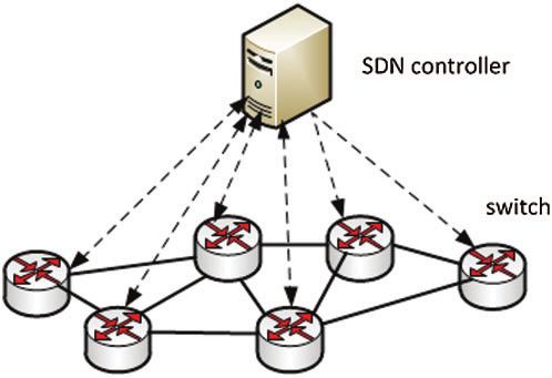
3750                                                                           CMC, 2021, vol.67, no.3

Accordingly, in the case of the vehicle placement density increase on the roads, the speed of node
movement and the throughput of highways will decrease. This raises the question of developing
new or making improvements in existing methods of Traffic Orchestration, which make it possible
to respond rapidly to the changes in the state of the transport network and ensure the most equal
load of channels.
     With the development of mobile communication technology, researchers have developed many
in-vehicle safety and non-safety applications, such as collaborative collision avoidance, route plan-
ning, autonomous driving, etc., but the in-vehicle network still faces many challenges due to the
difficulties in infrastructure deployment and management. For example, the number of connected
devices is increasing exponentially, the efficiency of resource utilization is low, and the traffic
flow is uneven. Other challenges include difficulties in geographical addressing, high mobility of
vehicles and unreliable connections, etc. The traditional vehicle network architecture uses special
algorithms in-vehicle components to monitor traffic density and plan routing paths to achieve
effective message transmission. However, the frequent interruption of vehicle communication,
heterogeneous network interfaces, and the growing demand for scalability, flexibility, safety and
reliability of the vehicle network has gradually revealed the drawbacks of a traditional vehicle
network. Also, the private ownership and tight coupling of hardware devices hinder the innovation
and development of computer networks. With an increase in the number of network devices
and the acceleration of network data transmission, traditional IP-based networks are becoming
increasingly difficult in deployment and management, and they can no longer meet the develop-
ment needs of future networks [2]. At the same time, the introduction of new services has also
created huge challenges for the construction, maintenance, and upgrade of the network, resulting
in increased operating costs, short equipment life cycles, and increasingly complex networks. SDN
points out the direction for solving the above problems. SDN represents an emerging network
model with the potential to join cellular networks and vehicle-mounted networks. First, SDN
separates control and forwarding functions, thus allowing researchers to directly program network
control and abstract infrastructure for applications and network services. Second, logically central-
ized control improves resource utilization efficiency. Third, programmability makes the network
more flexible, and applications would be able to select the most suitable wireless access interface to
transmit data. Therefore, the design of SDVN is an effective way to deal with vehicle application
requirements, manage dynamic network topologies, support network heterogeneity, and minimize
network management costs/design complexity [3].
     SDN is a routing technology that has emerged in recent years and is mainly used in wired
networks to improve their network bandwidth utilization. In recent years, research on software-
defined wireless networks has gradually become a hotspot. SDN can better realize the flexible
allocation and control of network resources, with obvious advantages in scalability and efficiency.
These technical advantages are in line with the characteristics of the vehicle network in terms of
node mobility, network dynamics, and network scale. Therefore, the introduction of SDN into the
Internet of Vehicles can better solve the current difficulties of the Internet of Vehicles. In particu-
lar, the centralized management and control concept of SDN based on the controller can solve the
difficulty of node coordination caused by the centerless and multiple changes of the Internet of
Vehicles. However, SDN is primarily used in wired networks, and its architecture considers wired
links and fixed equipment, with a stable network topology. The Internet of Vehicles is based on a
dynamic wireless network that comprises vehicle-to-vehicle (V2V) and vehicle-to-Roadside (V2R)
unit communication, whereas topology dynamic changes are not considered by general SDN.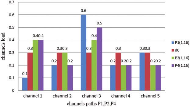
CMC, 2021, vol.67, no.3                                                                          3751

The problem. This is the main challenge of applying SDN in the vehicle network, in addition to
being the main goal of this paper. SDN can also be implemented in a dynamic topology [4].
    The rest of the paper is organized as follows. Section 2 provides a brief overview of TO
methods that currently exist in VANETs. The advantage of using multipath routing methods in
VANET based on TO has been justified. Section 3 proposes a modified TO method in SDVN.
The method for generating routing information with a minimum time for path reconfiguration
and dynamic rerouting of traffic flows has been developed and presented.

2 Related Work
     In general, Network Orchestration is a system for managing and optimizing network services.
Traffic Orchestration refers to the traffic engineering and management of the network traffic to
provide specified Quality of Service (QoS) parameters and an equal load of network channels.
Traffic Orchestration issues in SDN transport networks are connected with the increase in network
size and load on its channels. Real-time traffic engineering is essential to achieve even traffic bal-
ancing, fast disaster recovery, and congestion avoidance [5]. An update of the routing information
using well-known distributed routing techniques takes a significant amount of time and leads to
network jams and congestions. In this case, the centralized management of the transport network
is deemed most efficacious. One of the promising solutions to this challenge is the integration of
VANETs with software-defined networks (SDN) through Software-Defined Vehicular Networking
(SDVN). The convergence of SDN and VANET is known to solve common VANET issues,
including the balance of traffic load and dynamic path reconfiguration.
    A differential characteristic of SDN involved network management and organization. This
takes place at the software level through virtual switches alongside a central SDN controller as
shown in Fig. 1.

                  Figure 1: The structure of a software-defined network (SDN)

    This makes it possible to organize centralized and decentralized management for network
devices and increase the traffic engineering procedure’s functionality. In the case of the centralized
manner of path creation, the SDN controller holds all data on the network’s structure and
components, which facilitates optimization of paths as per specified metrics in the process of
path creation. SDN controller updates routing information for SDN switches by adjusting their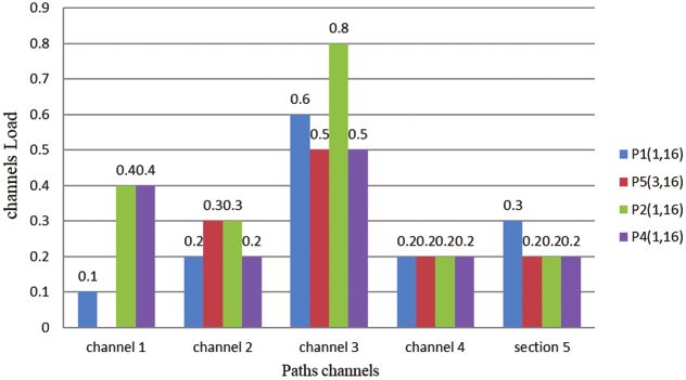
3752 CMC, 2021, vol.67, no.3
routing tables to select the optimal route as well as to secure minimal power consumption/channel
congestion [6].
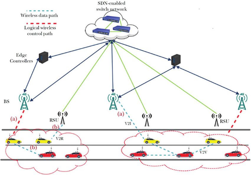
Figure 2: The structure of the SDVN network
The paper [7] shows a study of various methods and approaches to resolve the issues relating
to data traffic optimization in the context of the networks in question. The emphasis is placed
upon QoS, congestion control, and load balancing. Through this comparison to a typical network,
SDN’s main advantage is in centralized traffic orchestration by the SDN controller. This makes
it possible for better implementation of load balancing strategy. Compared to distributed traffic
engineering and balancing methods, the centralized method reduces the need for service informa-
tion exchange. The article [8] proposes a method for multipath routing in SDN based on MPLS
technology. Utilizing the SDN Controller’s centralized management manner of label allocation
helps improve the efficiency of the traffic orchestration process. In the multipath routing, MPLS
network routers generate labels for multiple possible paths to the destination. This makes it
possible to quickly redirect the traffic flows along an alternative route in case of road congestion.
In [9], a multipath routing algorithm is proposed to augment network performance by 10–15%
by diminishing the volume of service packets. This also lowers energy consumption by about 41%
and increases the maximum use of communication channels by 60% as compared to distributed
methods of traffic engineering and balancing. In [10], the authors propose a method for traffic
orchestration, which, due to the centralized method of generating routing information in theCMC, 2021, vol.67, no.3 3753
SDN controller and the use of multipath routing, makes it possible to make simplify the traffic
reconfiguration procedure and guarantee the most equal network load. The routing information
management is conducted by using the wave routing algorithm [11]. In this case, paths are
simultaneously created from all intermediate nodes to the final node. The study [12] deals with the
SDVN network design and considers the advantages of SDN technology utilization for building
transport networks. Fig. 2 shows the structure of the SDVN network.
3 Proposed Traffic Orchestration Procedure
3.1 Traffic Orchestration Criterion
The transport network in Fig. 3 is represented as a loaded graph G(V , C, D), where
V = (vi | i = 1, 2, .., m) the set of vertices denotes the set of switches (crossroads) of the transport
network; C = (ck (vi , vj ) | k = 1, 2, . . . , n)—the set of channels (sections) of the path between
adjacent crossroads vi and vj ; D = (dk | k = 1, 2, . . . , n)—loading channels ck (vi , vj ) of the path.
Figure 3: Transport network graph
A basic issue with well-known traffic engineering models has several flows undergoing redirec-
tion to the shortest path, thus resulting in load imbalance [13,14]. It is essential that nature and
volume be taken into consideration to handle this during traffic orchestration.
This is important for transport networks, in which a large load of the route channels leads
to traffic congestion. The speed of vehicles, including travel time, depends on the network load.
Different values of the path channel load also cause a decline in the average speed and through-
put of the entire transport network [1,2]. Therefore, while creating the next path pi (vs , ve ) it is
1
n
necessary to take into account the average load of its channels: di0 = dk [15].
n
k=1
As an example, consider the four shortest paths between vertices v1 and v16 (Fig. 3):
p1 (v1 , v16 ) = (v1 → v4 → v8 → v12 → v15 → v16 );
p2 (v1 , v16 ) = (v1 → v3 → v6 → v10 → v13 → v16 );
p3 (v1 , v16 ) = (v1 → v2 → v5 → v9 → v14 → v16 );
P4 (v1 , v16 ) = (v1 → v3 → v7 → v10 → v13 → v16 );3754 CMC, 2021, vol.67, no.3
Average path load p1 (v1 , v16 ) is d10 = 0,3.
Average path load p2 (v1 , v16 ) is d20 = 0,3.
Average path load p3 (v1 , v16 ) is d30 = 0,44.
Average path load p4 (v1 , v16 ) is d40 = 0,3.
The paths p1 (v1 , v16 ) , p2 (v1 , v16 ) p4 (v1 , v16 ) have equal average channel load.
Fig. 4 shows the load of channels paths p1 (v1 , v16 ), p2 (v1 , v16 ), p4 (v1 , v16 ) and their average
value d 0 .
Figure 4: Load of channels paths p1 (v1 , v16 ), p2 (v1 , v16 ), p4 (v1 , v16 ) and their average value d 0
Thereby, it is important to pick paths with the least average load and deviation of the path
load. In this case, the path p2 (v1 , v16 ) is chosen, since the path comprises more evenly loaded
channels with an equal average load of the channels.
The length of the path channels must be taken into account when choosing a path. The longer
the path channel, the more the congestion affects the load equability on the entire path.
To address this issue, the present work proposed to utilize the coefficient of equability of
loading the path channels as a criterion for choosing the path:
n
l (d
k k − d 0 )2
Mi (vs , ve ) = 1 − di0 + (1)
Li
k=1
where: n—number of path channels pi (vs , ve );
di0 —average load of path channels pi (vs , ve );
dk —channel load ck (vi , vj ) ∈ pi (vs , ve );
Li —path length pi (vs , ve );
lk —channel length ck (vi , vj ).
For example, consider a network with equal channel lengths.
In this case lk = Li /n.
For the path p1 (v1 , v16 ) the equability of the loading criterion M1 (v1 , v16 ) = 0,656.
For the path p2 (v1 , v16 ) the equability of the loading criterion M2 (v1 , v16 ) = 0,692.CMC, 2021, vol.67, no.3 3755
For the path p3 (v1 , v16 ) the equability of the loading criterion M3 (v1 , v16 ) = 0,536.
For the path p4 (v1 , v16 ) the equability of the loading criterion M4 (v1 , v16 ) = 0,642.
In this case, the chosen path is p2 (v1 , v16 ).
The equability of the path channels’ loading criterion depends on their length; for example,
if the channel c5,9 of the path p1 (v1 , v16 ) is three times longer than M1 (v1 , v16 ) = 0.643, then the
M1 (v1 , v16 ) criterion will be 1.3% lower.
Thus, the coefficient Mi makes it possible to optimize the traffic of vehicles by choosing the
least loaded equal path.
3.2 Traffic Orchestration Algorithm
Fig. 5 shows the flowchart of traffic orchestration. The SDN controller receives requests from
switches Qi (j) = {vi , vn , gj } to create a path between switches vi and vn , where: j—denotes the
number of the request from the switch vi ; gj —signifies the request priority Qi (j). The non-priority
request corresponds to gj = 0, and the priority one corresponds to gj = 1. Priority requests come
from special vehicles. Path requests are processed based on their priority and arrival time.
The paths are discovered from SDN controller path database. For every path pi (vs , ve ) there
is a corresponding set of vertices included in Vi = {vj | j = 1, .., m} and distance vectors Ri (vs , ve )
= {ve , va , Mi (vs , ve )}, where va —adjacent node towards the end node ve ; Mi (vs , ve )—channels load
equability coefficient.
Tab. 1 shows the values of the distance vectors for the paths:
p1 (v1 , v16 ) = (v1 → v4 → v8 → v12 → v15 → v16 );
p2 (v1 , v16 ) = (v1 → v3 → v6 → v10 → v13 → v16 );
p3 (v1 , v16 ) = (v1 → v2 → v5 → v9 → v14 → v16 ).
In this case, the path p2 (v1 , v16 ) is chosen.
The created path can fully or partially coincide with the path from the database. Here, we
will formulate the condition for the path presence between two arbitrary vertices of the transport
network graph.
Lemma 1. The condition for the path presence pj (vs , ve ) between two vertices {vs , ve }:
{vs , ve } ∩ {vk | k = 1, 2, . . . , m} = {vi vo}, (2)
where: vs —the initial vertex of the desired path;
ve —final vertex of the desired path;
{vk | k = 1, 2, . . . , m}—the set of vertices of the path pb ∈ P{pi | i = 1, 2, . . . , n};
P{pi (vs , ve ) | i = 1, 2, . . . , n}—the set of paths from the SDN controller database.
For example, consider finding the path pi (v3 , v13 ) between vertices v3 and v13 , and paths
presence in the database P{p1 (v1 , v16 ), p2 (v1 , v16 ), p3 (v1 , v16 ), p4 (v4 , v14 ), p5 (v3 , v14 ), p6 (v2 , v9 )}:
1. p1 (v1 , v16 ) = (v1 → v4 → v8 → v12 → v15 → v16 );
2. p2 (v1 , v16 ) = (v1 → v3 → v6 → v10 → v13 → v16 );
3. p3 (v1 , v16 ) = (v1 → v2 → v5 → v9 → v14 → v16 );
4. p4 (v4 , v14 ) = (v4 → v3 → v7 → v11 → v15 → v13 → v14 );
5. p5 (v3 , v14 ) = (v3 → v7 → v10 → v13 → v14 );
6. p6 (v2 , v14 ) = (v2 → v3 → v7 → v10 → v9 ).3756 CMC, 2021, vol.67, no.3
Figure 5: The flowchart of traffic orchestration algorithm
Table 1: Distance vector table for switch v1
No. Ri (vs , ve ) ve va Mi (vs , ve )
1 R1 (v1 , v16 ) v16 v4 0,656
2 R2 (v1 , v16 ) v16 v3 0,692
3 R3 (v1 , v16 ) v16 v2 0,536
4 R4 (v1 , v16 ) v16 v3 0,620CMC, 2021, vol.67, no.3 3757
In this case, condition (2) for the set of paths {p1 (v1 , v16 ), p2 (v1 , v16 ), p3 (v1 , v16 ), p4 (v4 , v14 ),
p5 (v3 , v14 ), p6 (v2 , v9 )} and the path pi (v3 , v13 ):
1. {v1 , v4 , v8 , v12 , v15 , v16 } ∩ {v3 , v13 } = ∅;
2. {v1 , v3 , v6 , v10 , v13 , v16 } ∩ {v3 , v13 } = {v3 , v13 };
3. {v1 , v2 , v5 , v9 , v14 , v16 } ∩ {v3 , v13 } = ∅;
4. {v4 , v3 , v7 , v11, v15 , v13 , v14 } ∩ {v3 , v13 } = {v3 , v13 };
5. {v3 , v7 , v10 , v13 , v14 } ∩ {v3 , v13 } = {v3 , v13 };
6. {v2 , v3 , v7 , v10 , v9 } ∩ {v3 , v13 } = {v3 }.
Consequently, three paths are discovered between the vertices v3 and v13 :
1. p1 (v3 , v13 ) = (v3 → v6 → v10 → v13 );
2. p2 (v3 , v13 ) = (v3 → v7 → v10 → v13 )
3. p3 (v3 , v13 ) = (v3 → v7 → v11 → v15 → v13 );
For the selected paths in the SDN controller, the metrics of their channels are updated, and
the value Mi (v3 , v13 ) is calculated for each path p1 (v3 , v13 ). Also, the distance vector table for the
switch v3 is created (Tab. 2).
Table 2: Distance vector table for switch v3
No. Ri (vs , ve ) ve va Mi (vs , ve )
1 R1 (v3 , v13 ) v13 v6 0,693
2 R2 (v3 , v13 ) v13 v7 0,680
3 R3 (v3 , vn ) v13 v7 0,536
Path data, along with their distance vectors, gets updated in the SDN controller database.
In this case, the path p1 (v3 , v13 ) is chosen, which forms part of the path p2 (v1 , v16 ) = (v1 → v3 →
v6 → v10 → v13 → v16 ) with value of M1 (v3 , v13 ) = 0,693.
3.3 New Paths Criterion
For {vs , ve } ∩ {vk | k = 1, 2, . . . , m} = {vs , ve } the SDN controller database does not contain any
information about path between vi and vn . In this case, routing information is generated based
on the modified Backward Wave algorithm [16]. The routing information is created in a wave
manner, beginning from the final vertex, similar to the distance-vector routing algorithm. The
routing information has been created sequentially between adjacent sets of vertices Vi+1 and Vi .
The creation starts with the vertex ve ∈ Vi . Simultaneously, further paths are developed between
the intermediate and final routers. Therefore, for each node vj ∈ Vi+1 of the path pj (vs , ve ) the
table of distance vectors is created Ri (vs , ve) = {ve , va , Mi (vs , ve )}. The vertex va ∈ Vi . The creation
ends when Vi+1 = {vs }. For the initial node vi of the path, the table of distance vectors is created
Ri (vs , ve ) = {ve , va , Mi (vs , ve )} along with the set of paths P = {pk (vi , ve ) | k = 1, .., m} between
vertices vi and ve .
Let’s consider an example of the routing information created between the vertices v1 and v16
(Fig. 3). For i=1 the set Vi = {v16 }, and the set Vi+1 = {v13 , v14 , v15 }.
Three paths are created: p1 (v13 , v16 ); p2 (v14 , v16 ); p3 (v15 , v16 ).
The path p1 (v13 , v16 ) contains the set of vertices {v13 , v16 }, M1 (v13 , v16 ) = 0.8.3758 CMC, 2021, vol.67, no.3
Tab. 3 shows the value of the distance vector for the vertex v13 in the direction of the
vertex v16 .
Table 3: Distance vector table for switch v13
No. Ri (vs , ve ) ve va Mi (vs , ve )
1 R1 (v13 , v16 ) v16 V16 0,8
The path p1 (v14 , v16 ) contains a set of vertices {v14 , v16 }, Mj (v14 , v16 ) = 0.4.
Tab. 4 shows the value of the distance vector for the vertex v14 in the direction of the
vertex v16 .
Table 4: Distance vector table for switch v14
No. Ri (vs , ve ) ve va Mi (vs , ve )
1 R1 (v14 , v16 ) v16 V16 0,4
The path p1 (v15 , v16 ) contains a set of vertices {v15 , v16 }, M1 (v15 , v16 ) = 0.7.
Tab. 5 shows the value of the distance vector for the vertex v15 in the direction of the
vertex v16 .
Table 5: Distance vector table for switch v15
No. Ri (vs , ve ) ve va Mi (vs , ve )
1 R1 (v15 , v16 ) v16 V16 0,7
For i = 2 the set Vi = {v13 , v14 , v15 }, and the set Vi+1 = {v9 , v10 , v11 , v12 }.
6 paths are created in the direction of the vertex v16 . The paths p1 (v9 , v16 ) and p2 (v9 , v16 ) are
created from the vertex v9 .
The path p1 (v9 , v16 ) contains the set of vertices {v9 , v13 , v16 }, M1 (v9 , v16 ) = 0.69.
The path p2 (v9 , v16 ) contains the set of vertices {v9 , v14 , v16 }, M2 (v9 , v16 ) = 0.447.
Tab. 6 shows the value of the distance vector for the vertex v9 in the direction of the
vertex v16 .
Table 6: Distance vector table for switch v9
No. Ri (vs , ve ) ve va Mi (vs , ve )
1 R1 (v9 , v16 ) v16 v13 0,69
2 R2 (v9 , v16 ) v16 v14 0,447CMC, 2021, vol.67, no.3 3759
In this case, the optimal path is p1 (v9 , v16 ).
Paths p1 (v10 , v16 ) and p2 (v10 , v16 ) are created from vertex v10 .
The path p1 (v10 , v16 ) contains the set of vertices {v10 , v13 , v16 }, M1 (v10 , v16 ) = 0.8.
The path p2 (v10 , v16 ) contains the set of vertices {v10 , v15 , v16 }, M2 (v10 , v16 ) = 0.725.
Tab. 7 shows the value of the distance vector for the vertex v10 in the direction of the
vertex v16 .
Table 7: Distance vector table for switch v10
No. Ri (vs , ve ) ve va Mi (vs , ve )
1 R1 (v10 , v16 ) v16 v13 0,8
2 R2 (v10 , v16 ) v16 v15 0,725
In this case, the optimal path is p1 (v10 , v16 ).
One path p1 (v11 , v16 ) is created from the vertex v11 . The path p1 (v11 , v16 ) contains the set of
vertices {v11 , v15 , v16 }, M1 (v11 , v16 ) = 0.625.
Tab. 8 shows the value of the distance vector for the vertex v11 in the direction of the
vertex v16 .
Table 8: Distance vector table for switch v11
No. Ri (vs , ve ) ve va Mi (vs , ve )
1 R1 (v11 , v16 ) v16 v15 0,625
One path p1 (v12 , v16 ) is created from the vertex v12 . The path p1 (v12 , v16 ) contains the set of
vertices {v12 , v15 , v16 }, M1 (v12 , v16 ) = 0.725.
Tab. 9 shows the value of the distance vector for the vertex v12 in the direction of the
vertex v16 .
Table 9: Distance vector table for switch v12
No. Ri (vs , ve ) ve va Mi (vs , ve )
1 R1 (v12 , v16 ) v16 v15 0,725
As a result, three disjoint paths pi (v1 , v16 ) with the maximum value of Mj (vi , vn ) are formed
for the vertex v1 (Tab. 10).
Table 10: Distance vector table for switch v1
No. Ri (vs , ve ) ve va Mi (vs , ve )
1 R1 (v1 , v16 ) v16 v4 0,656
2 R2 (v1 , v16 ) v16 v3 0,692
3 R3 (v1 , v16 ) v16 v2 0,5363760 CMC, 2021, vol.67, no.3
3.4 Load Balancing
While creating new paths or reconfiguring existing ones, the channels’ load of adjacent routes
is changing. This makes it imperative to fix adjacent routes to balance the load of the network
channels. The centralized method of generating routing information in the SDN controller elim-
inates the procedure of creating new paths when the network topology changes or its channels
are overloaded. The availability of several options of the distance vector at the vertices of the
selected path makes it possible to dynamically reconfigure the path considering the change in the
channel load. The SDN controller continuously monitors changes of the channel load, recalculates
the coefficient of equability for path channels, and incorporates changes made to the distance
vector tables on the switches. Based on the updated values of the distance vectors, it reconfigures
adjacent paths to load the network channels in a more even manner.
Algorithm 1: Correction of adjacent paths
Notations:
vs : vertex of the path begin;
ve : vertex of the destination;
pi (vs , ve ): selected (created) path from the vertex vs to the vertex ve
{(ck (vi , vj ) | k = 1, 2, . . . , n)}—set of channels of the selected (created) path pi (vs , ve );
P{pb (vs , ve ) | q = 1, 2, . . . , q}—multiple paths in the database of the SDN controller;
{ck (vj , vr ) | k = 1, 2, . . . , m}—the set of the link of the path pb (vi , vj ); ∈ P{pi (vs , ve ) | i = 1, 2, . . . , n};
Mi (vs , ve )—coefficient of equability of loading the path channel pi (vs , ve ).
1. begin
2. for i := 1 step 1 until n do
3. begin
4. for k := 1 step 1 until m do
5. begin
6. for j := 1 step 1 until q do
n} = ∅ go to 10; /∗ finding of adjacent paths ∗ /
7. if {cj | j = 1, 2, . . ., r} ∩ {ck | k = 1, 2, . . . ,
lk (dk − d0 )
n 2
8. Mj (vi , vn ) = 1 − d0 + /∗ adjustment coefficient of equability of loading the
Li
k=1
path channel pb (vs , vn ) ∈ P{pi (vs , vn ) | i = 1, 2, . . . , n}; ∗ /
9. end;
10. end;
11. end.
Consider load balancing when the load of the path channels is p1 (v5 , v15 ) = (v5 → v6 →
v10 → v15 ) at 0,4. In this case, the channel load is c2 (v6 , v10 ) = 0,7.
Fig. 6 shows the loading of path channels.
The path p1 (v5 , v15 ) is adjacent to paths p2 (v1 , v16 ) = (v1 → v3 → v6 → v10 → v13 → v16 ) and
p1 (v3 , v13 ) = (v3 → v6 → v10 → v13 ).
Criterion value M2 (v1 , v16 ) for the path p2 (v1 , v16 ) = (v1 → v3 → v6 → v10 → v13 → v16 ) is
attributed to the change in the channel load c6,10 decreases and becomes equal to M2 (v1 , v16 ) =
0,605 (Tab. 11). Here, the next path to be chosen is p1 (v1 , v16 ) = (v1 → v4 → v8 → v12 → v15 → v16 )
with the maximum criterion of equability of loading M1 (v1 , v16 ) = 0,656.CMC, 2021, vol.67, no.3 3761
Figure 6: The loading of path channels
Table 11: Distance vector table for switch v1
No. Ri (vs , ve ) ve va Mi (vs , ve )
1 R1 (v1 , v16 ) v16 v4 0,656
2 R2 (v1 , v16 ) v16 v3 0,605
3 R3 (v1 , v16 ) v16 v2 0,536
4 R4 (v1 , v16 ) v16 v3 0,620
For the path p1 (v3 , v13 ) the value C1 (v3 ) = 0,693 in the routing table of v3 switch will be
replaced with C1 (v3 ) = 0.556 (Tab. 12) due to the change in the channel load l6,10 .
Table 12: Distance vector table for switch v3
No. Ri (vs , ve ) ve va Mi (vs , ve )
1 R1 (v3 , v13 ) v13 v6 0,556
2 R2 (v3 , v13 ) v13 v7 0,680
3 R3 (v3 , v13 ) v13 v7 0,536
In this case instead of path p1 (v3 , v13 ) = (v3 → v6 → v10 → v13 ) the next path will be selected
p2 (v3 , v13 ) = (v3 → v7 → v10 → v13 ).
The existence of several alternative paths makes it possible to exclude the procedure of new
paths created during the movements of vehicles. For example, when a vehicle moves along the
path p2 (v1 , v16 ) = (v1 → v3 → v6 → v10 → v13 → v16 ), dynamic path reconfiguration will take place,
depending on the change in the nodes load. During channel l6,10 load changes, the vehicle from
v1 instead of the path p2 (v1 , v16 ) = (v1 → v3 → v6 → v10 → v13 → v16 ) will be redirected to the path
p1 (v1 , v16 ) = (v1 → v4 → v8 → v12 → v15 → v16 ); will be redirected to the path p2 (v3 , v16 ) = (v3 →
v7 → v10 → v13 → v16 ) when it is at the node v3 . When the channels c10,13 or c13,16 are overloaded,
the vehicle from the node v10 will be directed to the path p1 (v10 , v16 ) = (v10 → v15 → v16 ) instead
of the path p1 (v10 , v16 ) = (v10 → v13 → v16 ).3762 CMC, 2021, vol.67, no.3
By eliminating recalculation of the routes, the time for path reconfiguration is significantly
reduced, along with the probability of delays along the way.
4 Conclusion
This paper looks at Traffic Orchestration and proposes a related method, which examines the
particulars for an SDN organization, and more specifically, due to the central controller’s existence
within the network, which makes it possible to reduce the time of the set of routs creation and
to simplify the traffic orchestration procedure. The centralized manner of updating the routing
information in the SDN controller makes it possible to significantly reduce the time to update the
routing information and to simplify the process of traffic engineering, in comparison to distributed
routing algorithms.
The modified algorithm for the routing information creation is proposed, thus allowing simul-
taneous creation of a set of shortest paths not only between the initial and final nodes but also
between intermediate nodes of these paths. The existence of multiple routes allows the elimination
of delays and packet loss during traffic rerouting.
The standard for selecting the path from available path sets is proposed and justified, which
makes it possible to ensure a more equal load of channels during information transmission for a
given quality of service parameters.
Although more attention is being paid to Traffic Orchestration in VANETs, there are still
many issues that need to be thoroughly investigated.
Further improvements of Traffic Orchestration methods are predicated on predicting
and studying the nature of communication channel load utilizing artificial intelligence (AI)
technologies [17].
Acknowledgement: The authors extend their appreciation to the Deanship of Scientific Research
at King Saud University for funding this work through research Group No. (RG-1439-053).
Funding Statement: This work is supported by King Saud University.
Conflicts of Interest: The authors declare that they have no conflicts of interest to report regarding
the present study.
References
[1] J. C. Nobre, A. D. Souza, D. Rosario, C. Both, L. A. Villas et al., “Vehicular software-defined
networking and fog computing: Integration and design principles,” Ad Hoc Networks, vol. 82, no. 1,
pp. 172–181, 2019.
[2] C. Rostos, D. King, A. Farshad, J. Bird, L. Fawcett et al., “Network service orchestration standardiza-
tion: A technology survey,” Computer Standards and Interfaces, vol. 54, no. 4, pp. 203–215, 2017.
[3] I. F. Akyildiz, A. Lee, P. Wang, M. Luo and W. Chou, “Research challenges for traffic engineering in
software-defined networks,” IEEE Network, vol. 30, no. 3, pp. 52–58, 2016.
[4] O. S. Al-Heety, Z. Zakaria, M. Ismail, M. M. Shakir, S. Alani et al., “A comprehensive survey: Benefits,
services, recent works, challenges, security, and use cases for SDN-VANET,” IEEE Access, vol. 8,
pp. 91028–91047, 2020.
[5] B. Isong, T. Kgogo and F. Lugayizu, “Trust establishment in SDN: Controller and applications,”
International Journal of Computer Networks and Information Security, vol. 9, no. 7, pp. 20–28, 2017.
[6] A. A. AlZubi, M. Al-Maitah and A. Alaraifi, “A best-fit routing algorithm for non-redundant
communication in large-scale IoT based network,” Computer Networks, vol. 152, pp. 106–113, 2019.CMC, 2021, vol.67, no.3 3763
[7] A. Yasir, H. Chasib and Q. M. Zainab, “Analyzing methods and opportunities in software-defined
networks (SDN) for data traffic optimizations,” International Journal on Recent and Innovation Trends in
Computing and Communication, vol. 6, no. 1, pp. 75–82, 2018.
[8] D. Zbigniew, R. Grzegorz and C. Piotr, “MPLS-based reduction of flow table entries in SDN switches
supporting multipath transmission,” Computer Communications, vol. 151, pp. 365–385, 2020.
[9] K. Rajasekaran and K. Balasubramanian, “Energy conscious based multipath routing algorithm in
WSN,” International Journal of Computer Networks and Information Security, vol. 1, pp. 27–34, 2016.
[10] Y. Kulakoy, A. Kohan and S. Kopychko, “Traffic orchestration in data center network based on
software-defined networking technology,” in Int. Conf. on Computer Science, Engineering and Education
Applications, Kiev, Ukraine, pp. 228–237, 2019.
[11] Y. Kulakoy and K. Kogan, “The method of plurality generation of disjoint paths using horizontal
exclusive scheduling,” Advance Science Journal, vol. 10, pp. 16–18, 2014.
[12] A. A. AlZubi, “A new method oriented approach for forming multipath routing in cloud comput-
ing structure to accessing the protein folding information,” Journal of Medical Imaging and Health
Informatics, vol. 8, no. 4, pp. 801–804, 2018.
[13] M. T. Abbas, A. Muhammad and W. C. Song, “SD-IoV: SDN enabled routing for internet of vehicles
in road-aware approach,” Journal of Ambient Intelligence and Humanized Computing, vol. 11, pp. 1265–
1280, 2020.
[14] A. A. AlZubi, “Location assisted delay-less service discovery method for IoT environments,” Computer
Communications, vol. 150, pp. 405–412, 2020.
[15] M. T. Abbas and W. C. Song, “A path analysis of two-level hierarchical road, aware routing in
VANETs,” in IEEE Ninth Int. Conf. on Ubiquitous and Future Network, Milan, Italy, pp. 940–945, 2017.
[16] A. Abugabah, A. A. AlZubi, O. Alfarrai, M. Al-Maitah and W. S. Alnumay, “Intelligent traffic
engineering in software-defined vehicular networking based on multi-path routing,” IEEE Access, vol. 8,
pp. 62334–62342, 2020.
[17] A. A. AlZubi, “Bittorrent protocol for mobile health care system in hybrid P2P network architecture,”
Journal of Medical Imaging and Health Informatics, vol. 7, no. 2, pp. 508–513, 2017.You can also read