The Hubble Constant and the never-ending story of the expansion rate of the Universe - ESO Bruno Leibundgut

The Hubble Constant and the
 never-ending story of the
 expansion rate of the Universe

 Bruno Leibundgut
 ESO

11 January 2021 Bruno Leibundgut

Great Debate: What is the size of
 the Universe?
Presentations at the Annual Meeting of the
National Academy of Sciences in
Washington DC, 26. April 1920
 Harlow Shapley vs. Heber Curtis

 http://incubator.rockefeller.edu/geeks-of-the-week-harlow-shapley-heber-curtis/
11 January 2021 Bruno Leibundgut

Background
Expanding universe
 à expansion rate critical for cosmic evolution

 STScI
 Hubble 1929

11 January 2021 Bruno Leibundgut

Leading Theory of the Universe

11 January 2021 Bruno Leibundgut

Dealing with an
 expanding Universe
Cosmic Distances
Separate the observed distances ( ) into
the expansion factor ( ) and the fixed
part (called comoving distance)
 = 

 x

 x

11 January 2021 Bruno Leibundgut

Friedmann Equation
Time evolution of the scale
factor is described through
the time part of the Einstein equations
Assume a metric for a homogeneous and
isotropic universe and a perfect fluid
 ̇ ! 8 
 ! + != 
 3
 −1 0 0 0 # 0 0 0
 0 # 0 0 0 0 0
 !" = !" =
 0 0 # 0 0 0 0
 0 0 0 # 0 0 0 
11 January 2021 Bruno Leibundgut

Friedmann Equation
Put the various densities into the Friedmann equation
 ̇ ! !
 8 8 
 !
 = = − != " + # + $%& − !
 3 3 
 *+!"
Use the critical density &'() = ,-. ≈ 2 ⋅ 10/!0 /*
(flat universe), define the ratio to the critical density
 
 Ω=
 !"#$
Most compact form of Friedmann equation
 1 = Ω% + Ω& + Ω'() + Ω*
 *
with Ω* = − ! !
 11 January 2021 ( + Bruno Leibundgut

Dependence on Scale Parameter
For the different contents there were
different dependencies for the scale
parameter
 % ∝ ,- & ∝ ,. '() = 
Combining this with the critical densities
we can write the density as
 3 %& % ( % * % &
 = Ω' + Ω) + Ω+ + Ω,
 8 
and the Friedmann equation
 & = %& Ω' 1 + (
 + Ω) 1 + *
 + Ω+ + Ω, 1 + &

11 January 2021 Bruno Leibundgut

1927ASSB...47...49L
 History of 0
 Expansion rate by G. Lemaître (1927)

 Footnote!

 11 January 2021 Bruno Leibundgut

Intermezzo
 Age of the Universe
Matter-dominated universe has the
following age H (km/s/Mpc) t (yr)
 0 0

 500 1.30⋅109
 250 2.61⋅109
 2 100 6.52⋅109
 t0 =
 3H 0 80 8.15⋅109
 70 9.32⋅109
 60 1.09⋅1010
 50 1.30⋅1010
 30 2.17⋅1010

 – age of the Earth: 4.5⋅109 years
 – oldest stars: ~1.2⋅1010 years
11 January 2021 Bruno Leibundgut

History of 8
 https://www.cfa.harvard.edu/~dfabricant/huchra/hubble/

 2.6 ⋅ 10! 

 6.5 ⋅ 10! 

11 January 2021 Bruno Leibundgut

History of 8

 6.5 ⋅ 10! 

 13 ⋅ 10! 

11 January 2021 Bruno Leibundgut

History of 8

 6.5 ⋅ 10! 

 13 ⋅ 10! 

11 January 2021 Bruno Leibundgut

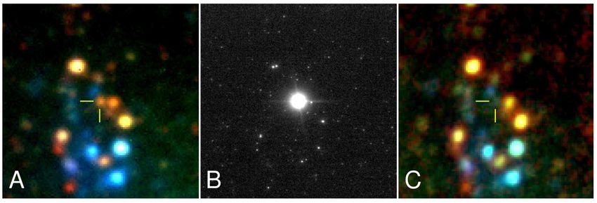
Extragalactic Distances
 Required for a 3D picture of the (local)
 universe

11 January 2021 Bruno Leibundgut

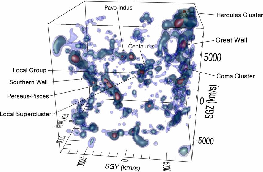
Extragalactic Distances
 The Astronomical Journal, 146:69 (14pp), 2013 September Courtois et al.

 Figure 8. Perspective view of the V8k catalog after correction for incompleteness and represented by three layers of isodensity contours. The region in the vicinity of
 the Virgo Cluster now appears considerably diminished in importance. The dominant structures are the Great Wall and the Perseus–Pisces chain, with the Pavo–Indus
 feature of significance.
 (A color version
11 January 2021of this figure is available in the online journal.) Bruno Leibundgut

Local Flows
Inhomogeneous mass distribution in the
local Universe 11

 Pomarède et al. 2020

 Figure 8. Flow streamlines seeded within the density unity contour of the Graziani et al. model. Flowlines
11 January 2021 Bruno Leibundgut
 proceed from seed position to one of three accumulation points associated respectively with the Shapley
 concentration, the Perseus Pisces filament, and the Great Attractor. Flow lines associated with seeds along

Measuring 8
 1974ApJ...190..525S Classical approach
 à distance ladder to reach (smooth)
 Hubble flow

 Sandage & Tammann 1974

11 January 2021 Bruno Leibundgut

Hubble Constant
Three different methods
 1. Distance ladder
 • Calibrate next distance indicator with the previous
 2. Physical methods
 • Determine either luminosity or length through
 physical quantities
 – Sunyaev-Zeldovich effect (galaxy clusters)
 – Expanding photosphere method in supernovae
 – Physical calibration of thermonuclear supernovae
 – Geometric methods, e.g. megamasers
 3. Global solutions
 • Use knowledge of all cosmological parameters
 – Cosmic Microwave Background

11 January 2021 Bruno Leibundgut

Michael Rowan-Robinson, in The Cosmological Dis- tances seems a real possibility.
 tance Ladder (1985) On the other hand, it is over 2000 years since Aristar-
 chus, and yet we are still unable to determine the scale of
 1. INTRODUCTION our universe to the satisfaction of the astronomical com-
 munity. By itself, this failure is not a serious transgression;
 Aristarchus of Samos, in the third century B.C., may it takes time to solve difficult problems. It is, however, a
 have been the first person to try measuring the size of his

 Classical Distance Ladder
 major embarrassment that the leading proponents in the
 universe when he estimated the ratio of the distances be- field have historically failed to agree within their stated
 tween the Sun and Moon. His efforts, which were later
 errors. If we dismiss the possibility of repeated oversights
 followed by the work of such well-known scientists as Er-
 in the analyses, then the most likely cause of the discrep-
 atosthenes, Hipparchus, Ptolemy, Copernicus, and Kepler,
 led to a set of reasonably good relative distances within the ancy is that the measurement uncertainties, internal and/
 solar system. With the advent of radar measurements in or external, have continually been underestimated.

Primary distance indicators (within the the mid-20th century, these relative values were placed on
 an absolute scale with unprecedented accuracy.
 Once outside the solar system, however, there is an
 It is this line of reasoning that led Rowan-Robinson
 (1985, 1988) to survey the field of extragalactic distance
 determinations, and we strongly encourage anyone inter-

Milky Way) enormous loss in the accuracy of distance determinations.
 Measurements of nearby stars and galaxies typically carry
 ested in this topic to consult these reviews. Other recom-
 mended reading on the subject includes Balkowski and

 – trigonometric parallax
 100 Mpc
 – proper motion ü 10 Mpc

 – apparent luminosity ~f~
 0
 1 Mpc

 • main sequence 100 Kpc

 10 Kpc
 • red clump stars
 ë 1 Kpc
 >»
 • RR Lyrae stars 1
 100 pc

 • eclipsing binaries
 Pathways to Extragalactic Distances
 • Cepheid stars Fig. 1—In this diagram we illustrate the various modem routes which may be taken to arrive at H and the genealogy and approximate distance range
 0
 Jacoby
 for each of the indicators involved. Population I indicators appear on the left-hand side and Population IIet al.right-hand
 on the 1992side. The distance increases
 logarithmically toward the top of the diagram. The following abbreviations have been used to conserve space: LSC—Local Super Cluster; SG—
 Supergiant; SN—Supernovae; B-W—Baade-Wesselink; PNLF—Planetary-Nebula Luminosity Function; SBF—Surface-Brightness Fluctuations;
 GCLF—Globular-Cluster Luminosity Function; —parallax.
11 January 2021 Bruno Leibundgut

Classical Distance Ladder

 Gruber Cosmology Prize
 Secondary distance AA48CH17-Freedman ARI 23 July 2010 16:29

 indicators (beyond the
 Local Group) 3
 I-band Tully-Fisher
 Fundamental plane
 79 72
 65

 – Important check Surface brightness
 Supernovae Ia

 Velocity (km s–1 × 10 4 )
 2 Supernovae II
 • Large Magellanic Cloud
 – Tully-Fisher relation
 1

 – Fundamental Plane
 ophys. 2010.48:673-710. Downloaded from www.annualreviews.org

 – Supernovae (mostly SN Ia) Freedman & Madore 2010
 Southern Observatory on 10/30/14. For personal use only.

 0

 – Surface Brightness 100 v > 5,000 km s–1 H0 = 72

 H0 (km s –1 Mpc –1)
 80
 Fluctuations 60

 40

 0 100 200 300 400
 Distance (Mpc)

 Figure 10
 11 January 2021 BrunoetLeibundgut
 Graphical results of the Hubble Space Telescope Key Project (Freedman al. 2001). (Top) The Hubble
 diagram of distance versus velocity for secondary distance indicators calibrated by Cepheids. Velocities are
 corrected using the nearby flow model of Mould et al. (2000). Dark yellow squares, Type Ia supernovae;

Hubble Constant
 HUBBLE
 HUBBLE CONSTANT:
 CONSTANT: REBUILD
 REBUILD DISTANCE
 DISTANCE LADDER
 LADDER
Calibration of M(SN Ia @ max)
 Eliminating sources of systematic error between anchor and calibrator:
 Eliminating sources of systematic error between anchor and calibrator:
 1) use same instrument 2) same Cepheid parameters (Period,Z) 3) better anchor
Distance ladder
 1) use same instrument 2) same Cepheid parameters (Period,Z) 3) better anchor

 PAST DISTANCE LADDER (100 Mpc) NEW LADDER (100 Mpc)
 PAST DISTANCE LADDER (100 Mpc) NEW LADDER (100 Mpc)
 11% error 4%
 11% ____
 error 4%
 ________ error
 ____ error____
 ____
 ____
 ____ Hubble Flow
 Hubble Flow Hubble Flow
 Hubble Flow 1% # Modern, distant SNe Ia
 1% # Modern, distant SNe Ia
 3% # Modern, local hosts 1%
 3% # Modern, local hosts 1%
 2%
 3.5% SN Ia hosts, 2%
 3.5% SN Ia hosts,
 Metallicity change
 Metallicity change

 Calibrator
 Calibrator
 4% long to short Period Cepheids
 4% long to short Period Cepheids

 NA NA
 4.5% Ground to HST
 4.5% Ground to HST

 5% Anchor: LMC 3% Anchor:
 5% Anchor: LMC 3% Anchor:
 NGC4258 Adam Riess
 NGC4258

11 January 2021 Bruno Leibundgut

The Astrophysical Journal, 826:56 (31pp), 2016 July 20 Riess et al.

 Hubble Constant
Supernova Ia
Hubble diagram

 Riess et al. 2016

11 January 2021 Figure 10. Complete distance ladder. The simultaneous agreement of pairs of geometric and Cepheid-based distances (lower left), Cepheid Bruno Leibundgut
 and SN Ia-based distances
 (middle panel) and SN and redshift-based distances provides the measurement of the Hubble constant. For each step, geometric or calibrated distances on the x-axis
 serve to calibrate a relative distance indicator on the y-axis through the determination of M or H0. Results shown are an approximation to the global fit as discussed in

 8 with Supernovae
• Local calibrators (calibrate the Cepheid L-P rel.)
 – Large Magellanic Cloud
 • 1% accuracy with eclipsing binaries (Pietrzyński et al. (2019)
 – Maser in NGC 4258
 • 3% accuracy (Humphreys et al. 2013)
 – geometric distances (parallaxes) to nearby Cepheids
• Extinction
 – absorption in the Milky Way and the host galaxy
 – corrections not always certain
• Peculiar velocities of galaxies
 – typically around 300 km/s
 11 January 2021 Bruno Leibundgut

SN Classification

11 January 2021 Bruno Leibundgut

The Extremes of Thermonuclear Supernovae 3

 Type Ia Supernovae
 The Extremes of Thermonuclear Supernovae 3

Variations on a theme Taubenberger 2017

 – critical parameters?
 • nickel mass
 • ejecta mass
 • explosion energy(?)
 • explosion mechanism?
 • progenitor evolution?

 Fig. 1 Phase space of potentially thermonuclear transients. The absolute B-band magnitude at peak
 is plotted against the light-curve decline rate, expressed by the decline within 15 d from peak in
11 January 2021 the B band, D m15 (B) (Phillips, 1993). The different classesBruno
 of objects discussed in this chapter
 Leibundgut
 are highlighted by different colours. Most of them are well separated from normal SNe Ia in this
 space, which shows that they are already peculiar based on light-curve properties alone. The only

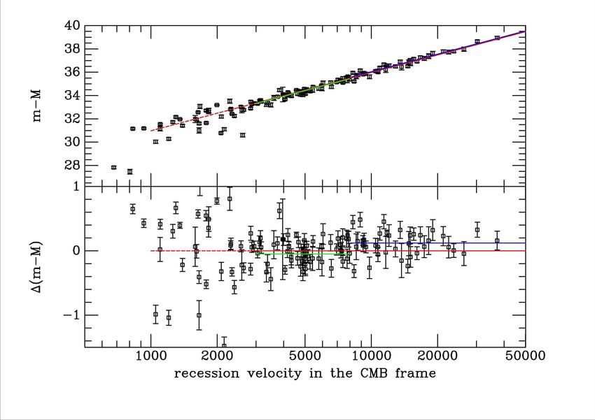
Hubble Constant
SN Hubble diagram
 − = 5 log + 25 − 5 log !
 Proves is constant
 Direct connection of and
 $
 Leibundgut

11 January 2021 Bruno Leibundgut

SNe Ia Hubble Diagram (NIR)
9 calibrators + 27 Hubble flow SNe
Dhawan et al. 2018
 " = (72.8 ± 1.6 ± 2.7 ) #$ #$ The Astrophysical Journal, 826:56 (31pp), 2016 July 20 Riess et al.

 Riess et al. 2016

 Figure 10. Complete distance ladder. The simultaneous agreement of pairs of geometric and Cepheid-based distances (lower left), Cepheid and SN Ia-based distances
 (middle panel) and SN and redshift-based distances provides the measurement of the Hubble constant. For each step, geometric or calibrated distances on the x-axis
 serve to calibrate a relative distance indicator on the y-axis through the determination of M or H0. Results shown are an approximation to the global fit as discussed in
 the text.

 with blending higher than the inner region of NGC 4258 to the relation. However, some insights into these systematics may be
 remaining 13. The difference in the mean model residual garnered by replacing the NIR-based Wesenheit magnitude, mHW ,
 distances of these two subsamples is 0.02±0.07 mag, with the optical version used in past studies (Freedman et al.
 providing no evidence of such a dependence. 2001), mIW = I - R (V - I ), where R≡AI/(AV − AI) and the
 value of R here is ∼4 times larger than in the NIR. The
 advantage of this change is the increase in the sample by a little
 4.2. Optical Wesenheit Period–Luminosity Relation over 600 Cepheids in HST hosts owing to the greater FOV of
 The SH0ES program was designed to identify Cepheids from WFC3/UVIS. Of these additional Cepheids, 250 come from
 optical images and to observe them in the NIR with F160W to M101, 94 from NGC 4258, and the rest from the other SN hosts.
 reduce systematic uncertainties related to the reddening law, its In Table 8 we give results based on Cepheid measurements of
 free parameters, sensitivity to metallicity, and breaks in the P–L mIW instead of mHW for the primary fit variant with all four

 17

11 January 2021 Bruno Leibundgut

Problem solved?
New discrepancy
between the Freedman 2017

measurements of
the local H0
(distance ladder)
and early universe
(CMB)
Indication of an
incomplete model
of cosmology?
 11 January 2021 Bruno Leibundgut

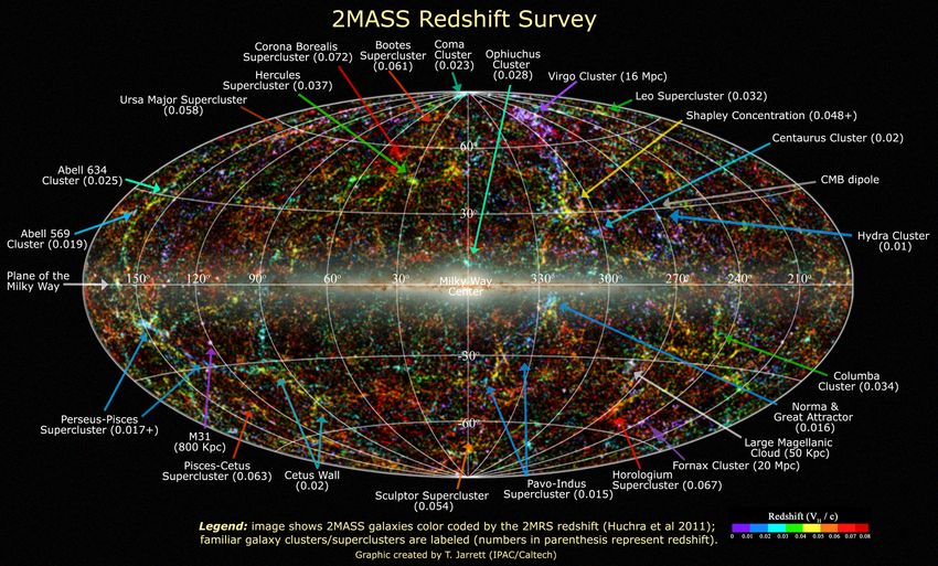
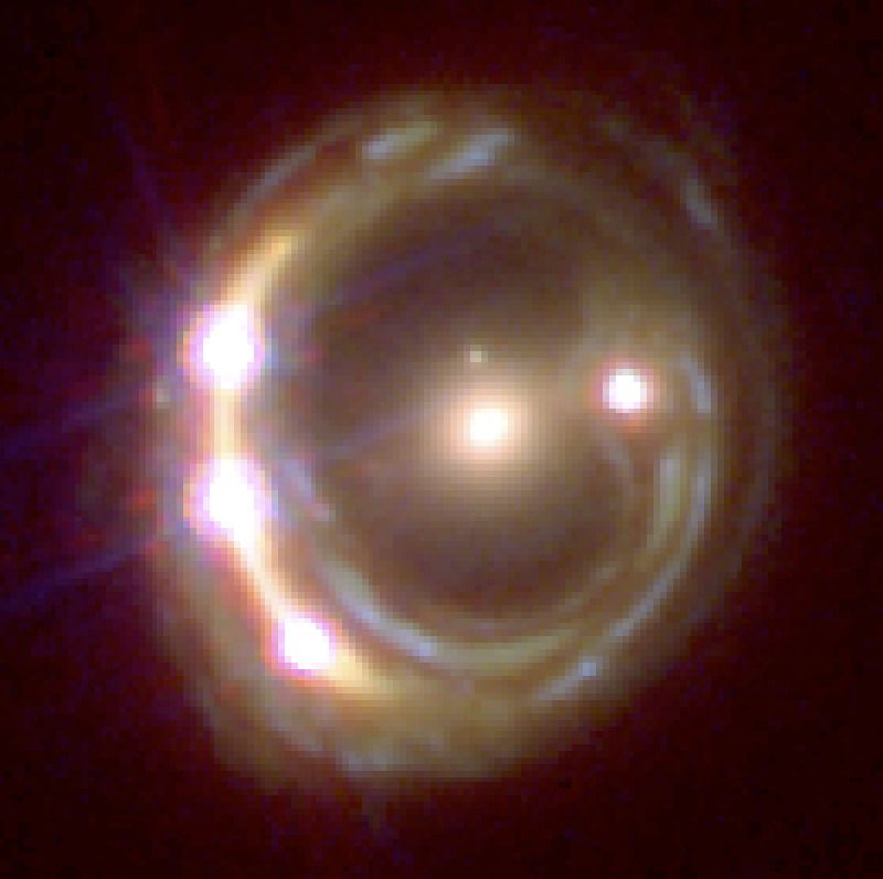
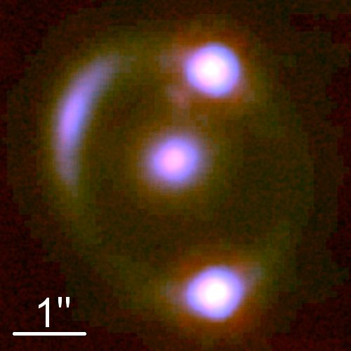
Sherry Suyu (J. Wiedersich / TUM)

 Gravitational Lenses
 Time delays in lensed quasars H0LiCOW XI
 time delays us
 18 K. C. Wong et al. fit a function t
 the time shift
 (Tewes et al.
 are made pub
 PyCS2 , which
 lays uncertain
 age was teste
 Wong et al. 2020 COSMOGRA
 ric noise in a
 1" 1" Bonvin et al. (
 curve-shifting
 (a) B1608+656 (b) RXJ1131 1231
 precision of ⇠
 Tewes et
 RXJ1131 123
 1.5% precision
 also measured
 time delay be
 111.3 ± 3 days
 (2019) re-anal
 and independ
 this result. Fo
 1" surement was
 of the COSM
 (c) HE 0435 1223 (d) SDSS 1206+4332 longest time d
 Recently,
 high-cadence
 campaign can
 from the intri
 tions of the qu
 than the typic
 sible to disent
 the microlensi
 were used for
 time delays at
 1" results are in a
 decade-long C
 (e) WFI2033 4723 (f) PG 1115+080 in the final es
 Figure 1. Multicolor images of the six lensed quasars used in The rema
 our analysis. The images are created using two or three imag- itored by Fass
 ing bands in the optical and near-infrared from HST and/or tions from the
 Figure 12. Comparison of H0 constraints for early-Universe and late-Universe probes in a flat ⇤CDM cosmology. The early-Universe ground-based AO data. North is up and east is to the left. independent t
 Images for B1608+656, RXJ1131 1231, HE 0435 1223, and measured to a
 probes shown here are from Planck (orange; Planck Collaboration et al. 2018b) and a combination of clustering and weak lensing data,
 WFI2033 4723 are from H0LiCOW I.
 BAO, and big bang nucleosynthesis (grey; Abbott et al. 2018b). The late-Universe probes shown are the latest results from SH0ES (blue; A compli
 Riess et al. 2019) and H0LiCOW (red; this work). When combining the late-Universe probes (purple), we find a 5.3 tension with Planck. delays to a c
 crolensing tim
 lenses to analyze first, as there may be systematics that de-
 11 January 2021 Bruno Leibundgut
 pend on such factors, and we want to account for them in
 estimation of
 which predicts
 7 SUMMARY mating our uncertainties and are able to control systematic our analysis (see Ding et al. 2018, who attempt to address
 disk from a ce
 these issues based on simulated data).

 8 Summary

 Bonvin and Millon
 https://doi.org/10.5281/zenodo.3635517

11 January 2021 Bruno Leibundgut

SN by volume

Type II Supernovae Ia
 24%

 II
 57%
 Ibc

• Core-collapse explosions of 19%

 massive, red-supergiant stars

 Mattila et al. 2010
• Peak absolute mags between -16 and -18
 → observable up to z ≈ 0.4
• Most common type of SN by volume
11 January 2021 Bruno Leibundgut

Physical parameters of core
 collapse SNe
Light curve shape and the velocity
evolution can give an indication of the total
explosion energy, the mass and the initial
radius of the explosion
 Observables:
 • length of plateau phase Δt
 • luminosity of the plateau LV
 • velocity of the ejecta vph

 • E µΔt4·vph5·L-1
 • MµΔt4·vph3·L-1
 • R µΔt-2·vph-4·L2

11 January 2021 Bruno Leibundgut

Expanding Photosphere Method

 1974ApJ...193...27K
Modification of Baade-Wesselink method
for variable stars
• Assumes
 – Sharp photosphere
 à thermal equilibrium
 – Spherical symmetry
 à radial velocity
 – Free expansion

 Kirshner & Kwan 1974
11 January 2021 Bruno Leibundgut

EPM: it’s all in the spectra

 C. Vogl
 Image: Héloïse Stevance

11 January 2021 Bruno Leibundgut

Expanding Photosphere Method
 - 
 = = & ; = − % + % ; . = ( − % )
 - + 

• R from radial velocity
 – Requires lines formed close to the photosphere
• D from the surface brightness of the black
 body
 – Deviation from black body due to line opacities
 – Encompassed in the dilution factor "

11 January 2021 Bruno Leibundgut

0.15 0.15

 Mpc

 Mpc
 d

 d
 ⇥

 ⇥
 q†

 q†
 2v

 2v
 c=

 c=
 0.10 0.10

 0.05
 Expanding Photosphere 0.05

 0.00

 40 20
 Method 0 20
 Epoch⇤ relative to discovery (rest frame)
 PS1-13wr

 40
 0.00

 40 20 0 20
 Epoch⇤ relative to discovery (rest frame)
 PS1-13wr

 40

 Θ 1
 = ( − using
Fig. C.3. Distance fit for PS1-13wr $ ) ⇣BVI as given in Hamuy et al. (2001; left panel) and Dessart & Hillier (2005; right panel). The diamond
 of % through which the fit is made.
markers denote values
 Gall et al. 2018
 0.14 0.14
 B: DL = 357 ± 43 Mpc B: DL = 409 ± 49 Mpc
 0.12
 V: DL = 349 ± 34 Mpc 0.12
 V: DL = 399 ± 39 Mpc
 Θ/v

 Θ/v
 I: DL = 366 ± 29 Mpc I: DL = 419 ± 33 Mpc
 0.10 0.10

 0.08 0.08
 ⇤

 ⇤
 Mpc

 Mpc
 d

 d
 ⇥

 ⇥
 q†

 q†
 2v

 2v
 0.06 0.06
 c=

 c=
 0.04 0.04

 0.02 0.02

 0.00 PS1-12bku 0.00 PS1-12bku
 0 10 20 30 40 0 10 20 30 40
 Epoch⇤ relative to discovery (rest frame) Epoch⇤ relative to discovery (rest frame)

 t-t0⇣BVI as given in Hamuy et al. (2001; left panel) and Dessart & Hilliert-t
Fig. C.4. Distance fit for PS1-12bku using (2005;
 0 right panel). The diamond
markers denote values of through which the fit is made.

 0.12 B: DL = 474 ± 54 Mpc 0.12 B: DL = 505 ± 58 Mpc
 11 January 2021
 V: D = 440 ± 47 Mpc V: DL = 469 ± 50 Mpc
 Bruno Leibundgut
 L

 0.10 I: DL = 463 ± 47 Mpc 0.10 I: DL = 494 ± 50 Mpc

Preliminary Results
 Consistent results
 – not independent as local calibration required
 E. E. E. Gall et al.: An updated Type II supernova Hubble diagram
 Gall et al. 2018
 42 42
 EPM SCM
 PS1-13bmf
 PS1-13bmf
 40 1000 40 PS1-14vk 1000
 PS1-14vk
 LSQ13cuw
 38 LSQ13cuw 38

 36 36

 DL [Mpc]

 DL [Mpc]
 100 100
µ

 µ
 34 34

 32 32 This work:
 This work: P09 D05 – Hb
 30 E96 D05 – Fe 10 30 P09 culled Phot – Hb 10
 H0 = 70 ± 5 km s 1 Mpc 1 J09 D05 – Hb H0 = 70 ± 5 km s 1 Mpc 1 O10 D05 – Fe
 Wm = 0.3, WL = 0.7 B14 Wm = 0.3, WL = 0.7 A10 Phot – Fe
 28 28
 0.001 0.002 0.005 0.01 0.02 0.05 0.1 0.2 0.3 0.001 0.002 0.005 0.01 0.02 0.05 0.1 0.2 0.3
 z z

Fig. 7. SN II Hubble diagrams using the distances determined via EPM (left panel) and SCM (right panel). EPM Hubble diagram (left): the
distances derived for our sample (circles) use the dilution factors from Dessart & Hillier (2005). The di↵erent colours denote the absorption line that
was used11to January
 estimate2021
 the photospheric velocities (Fe ii 5169 – red; H – blue). We also included EPM measurementsBruno Leibundgut
 from Eastman et al. (1996,
E96), Jones et al. (2009, J09) and Bose & Kumar (2014, B14). The solid line corresponds to a ⇤CDM cosmology with H0 = 70 km s 1 Mpc 1 ,

Expanded Photosphere
 Method Reloaded
• Use individual atmospheric models for
 the spectral fits
 – use of the TARDIS radiation transport model
 – absolute flux emitted
• Accurate explosion date
 – accurate zero point
• At least 5 epochs per supernova

11 January 2021 Bruno Leibundgut

Atmosphere
Models

TARDIS fits for
different epochs

 Vogl et al. 2020

11 January 2021 Bruno Leibundgut

Distance Determination
 G H
Slope is inverse distance: = ( − J )
 ' I"

 Vogl et al. 2020

11 January 2021 Bruno Leibundgut

adH0cc
“accurate determination of H0 with core-collapse supernovae”
(Flörs, Hillebrandt, Kotak, Smartt, Spyromilio, Suyu, Taubenberger, Vogl)
• Use the Expanding Photosphere Method to ~30 Type II
 supernovae in the Hubble flow (0.03

20. Past and ongoing observational programs

 SN 2019vew

 adH0cc
Critical observables
 – time of explosion +12.0 d

 – spectral coverage

 F⁄ + const.
 +15.0 d

 • before max until +19.0 d

 well into the plateau
 +22.0 d
 – photometry
 • simultaneously to +25.0 d

 spectroscopy +36.0 d

 C. Vogl 2020
 4000 5000 6000 7000 8000 9000 10000
 Wavelength [Å]

11 January 2021 Bruno Leibundgut
 Figure 20.4.: Time series of VLT+FORS2 spectra of SN 2019vew. Phases are reported relative

VLT– status FORS2

 C. Vogl (2020)
11 January 2021 Image:Bruno Leibundgut
 ESO/Y. Beletsky

Conclusions
Hubble constant sets absolute scale
(and age) of the universe
 – Past conflicts resolved
 • Age of Universe is bigger than age of
 the Earth
 – recognition of different stellar populations
 • Age of Universe bigger than oldest stars
 – cosmological constant

 11 January 2021 Bruno Leibundgut

Conclusions
Current discrepancy of 4 to 5 between
 – ! measured locally (distance ladder) and
 – ! measured at z=1100 (CMB)
Significance?
 – systematics based on Cepheid calibration
Extreme accuracy required
Independent measurements needed
 – Expanding Photosphere Method

11 January 2021 Bruno Leibundgut