The relationship between current load and temperature for quasi-steady state and transient conditions
←
→
Page content transcription
If your browser does not render page correctly, please read the page content below
The relationship between current load and temperature
                    for quasi-steady state and transient conditions
                             Bernard R. Lyon Jr., Gary L. Orlove, and Donna L. Peters

                  Infrared Training Center, 16 Esquire Road, North Billerica, MA 01862-2598

                                                          ABSTRACT
 Infrared thermographers involved in predictive maintenance programs often use temperature measurement as a means of
 quantifying the severity of a problem. Temperature is certainly an important factor in evaluating equipment. However, if you
 follow guidelines that are based solely on absolute temperature measurement - or on a temperature rise (Delta T) — you run
 the risk of incorrectly diagnosing your problems. The consequences of such actions can lead to a false sense of security,
 equipment failure, fire, and even the possibility ofpersonal injury. Understanding the additional factors involved in diagnosis
 is essential for obtaining productive results. One of these factors is the load or current flowing through conductors. The load
 can have a drastic effect on the temperature of a component. Changing loads can cause additional concerns because
 temperature changes lag behind load changes. The purpose of this paper is to illustrate the relationship between load and
 temperature of a faulty connection. The thermal response of a changing load is also investigated.

 Keywords: Keywords: infrared, thermography, predictive maintenance, temperature, current, load, electrical inspections,
 fused cut out, switch

                                                    1. INTRODUCTION
 An experienced thermographer can inspect numerous components quickly with an infrared imager. In addition he or she can
 make an informed recommendation to prioritize repair schedules based on the condition of the equipment rather than
 according to a timetable. For the most part, these recommendations are based on temperature criteria. In a perfect world,
 electrical equipment supply manufacturers would provide these threshold criteria. Currently, very little information is
 available from the manufacturers. Thermographers are therefore faced with the problem of deciding how to classify
 equipment as properly functioning, requiring more frequent monitoring, or critical. The problem lies in the fact that there is a
 wide variety of equipment in the field that was produced by many manufacturers and installed as long as 30 years ago.
 Thermally characterizing this equipment would be resource intensive. To add to the problem, variability in the conditions
 under which the equipment is surveyed will have dramatic effects on the results. Several independent organizations have
 begun to address this need by publishing severity criteria recommendations including the International Testing Association
 and the Electric Power Research Institute.

 The printed word carries a lot of weight, and many people are inclined to follow established guidelines, confident that they
 are "going by the book." Inevitably, an anomaly will be found and classified as normal; or at the most, requiring
 maintenance when it is convenient to do so. This anomaly then causes the equipment to fail even though all the guidelines
 were followed to the letter. So, what went wrong? There are many factors that can cause this situation. Some ofthese factors
 are: load, wind, solar heating, emissivity, variations in material properties (i.e. thermal conductivity), and the structure of the
 target. All too often in the tables, load is ignored, loosely defmed, or grouped in with other parameters, such as equipment
 type, temperature ratings, etc. The following five aspects relating to the importance of current load are examined in this
 paper: temperature as a severity criteria, using delta-T's vs. absolute temperatures, compensation equations, transient vs.
 steady state evaluation, and minimum load requirements for accurate thermograms.

                                   2. TEMPERATURE AS A SEVERITY FACTOR
 How hot is too hot? New thermographers ask this question often. It is a legitimate inquiry. If a sincere effort is made to
 conduct a thermographic inspection in the most efficient manner, it is necessary to locate and repair problems that truly need
 corrective measures; and, to avoid misdiagnosis of problems, so that efforts are not expended in fixing components that are
 working properly. So, thermographers are constantly searching for a means of identifying real problems. It is inevitable that
 temperature is going to be one of the factors, if not the primary factor, involved in the identification of problems. The

                                                                   In Thermosense XXII, Ralph B. Dinwiddie, Dennis H. LeMieux, Editors,
62                                                                        Proceedings of SPIE Vol. 4020 (2000) • 0277-786X!OO/$1 5.00
classical approach to the identification of faults has been the utilization of a criteria table with temperatures and
characterizations, grade assignments, or suggested actions. Here is a typical guideline, from the International Testing
Association Maintenance Testing Specifications, 1997 (NETA MTS-1997):
Possible deciency; warrants
1°C — 3°C 0°C — 10°C
investigation
4°C — 15 °C
Indicates orobable deficiency; repair as
11°C — 20°C
time permits
Monitor continuously until corrective
--- 22°C — 40°C
measures can be accomplished
> 16°C > 40°C Major discrepancy; repair immediately
Table 1 . Thermographic Survey - Suggested Actions Based on Temperature Rise
Temperature specifications vary depending on the exact type of equipment. Even in the same class of equipment
(i.e. cables) there are various temperature ratings. Heating is generally related to the square of the current;
therefore, the load current will have a major impact on temperature rise. In the absence of consensus standards for
temperature rise, the values in this table will provide reasonable guidelines.
We have examined several guidelines and standards used by various industries and utility companies and, with respect to
current load, most oftheir procedures have statements similar to the following:
". . . Corrective measures required as scheduling permits or ASAP, depending on the class of load and the severity
oftemperature rise in this range."
". . . The criteria are based on fully loaded circuits."
". . . Decision as to priorities and order of maintenance should be determined by the degree of temperature rise and
' criticality of the equipment or process involved."
We are confident that in the future we can expect to see further refmement of tables, including more variables, such as load,
wind, thermal insulating factors (elbows, splices) etc.
3. TEMPERATURE RISE
A single temperature reading, of and by itself, is usually insufficient information with respect to diagnosing a potential
problem. One must take into account the environmental temperature as well as any other heat loss or gain that can take place.
In a transformer heat is generated by eddy currents, (in the core) and by resistance, (in the windings). A correct understanding
of the equipment being inspected is essential if one is to make a proper thermographic diagnosis. And, as we shall see,
understanding how current loads contribute to temperature is an integral factor in evaluating the severity of a fault.
4. HOW RESISTANCE GENERATES HEAT
To understand why current load is important with respect to temperature measurements, it is necessary to understand how
heat is generated in electrical equipment. There is a fairly straightforward relationship between current I, resistance R, and
power P. The power generated in a circuit is the product ofthe current squared and the resistance. Or:
P=12R. (1)
All current carrying conductors used in electrical equipment have some resistance. Therefore, power will be generated in any
conductor carrying a load. Properly operating electrical equipment will have a thermal signature that depends on the type of
equipment, environmental temperatures, current load, and how long the equipment has been under load. In general,
conductors that have been carrying a reasonable current load continuously, over an extended period of time, will look hotter
than their surroundings. It is normal for conductors to heat up. Most guidelines, as indicated, suggest that thermographic
surveys should be conducted at maximum load, or at some reasonable percentage of maximum. Most electrical faults are
63essentially high resistance paths, caused by loose connections, corrosion, etc. If we assume that resistance remains fairly
constant, consider what happens as the load increases.
. If the load doubles, the power increases by a factor of four.
. Ifthe load triples, the power increases by a factor of nine.
. If the load quadruples, the power increases by a factor of sixteen.
These values clearly indicate the importance of current load with respect to power dissipated through a high resistance path.
To quantify and examine this more closely, a special test fixture was constructed. The resistance was kept constant, current
load was varied, and temperature measurements were taken.
5. TEST FIXTURE
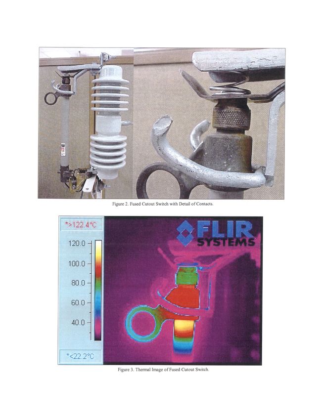
In order to simulate a real electrical fault, a fused cutout switch was used. The fuse and copper arc-shorting rod were removed
from the fuse tube. A heating element was installed in the cap end of the fuse holder; simulating a high resistance contact
between the fuse cap and the top contact. Thermographers experienced in inspecting these devices have stated that they
cannot tell the difference between the simulated fault and a real one.
Figure 1. Test Setup
The heating element was connected to a BK isolated variable AC power supply. The output was adjusted from 0 to 120 volts
AC. A meter on the supply was used to measured voltage or current, selected by using switches. A current probe, connected
to a digital multimeter, was used to measure the current. A type K thermocouple was used to monitor the temperature at the
contacts. Thermographic temperature data were taken with a Fur ThennaCam PM 390 and saved on a PCMCIA card as 12
bit TIFF files. TherMonitor 95 Pro thermal image processing and Plot 95 were used to analyze the thermal images. An area
on the cap of the fuse clip was outlined and the maximum, mean and minimum temperatures were recorded for each image.
6465
6. THERMAL DATA FROM LOAD CHANGES
 The intent of this experiment was twofold: First, to observe the effects of different loads under conditions where the
 apparatus has reached steady state and second, to observe the transient effect of a load change. The load was changed and the
 apparatus was given ample time to reach a state ofthermal equilibrium. An increase or decrease in load of25% was found to
 stabilize well within one hour. For this experiment, we defmed a full load condition when the output voltage was set at 120
 volts AC. As observed below, this resulted in a current flow of 0.23 amperes. And, as expected, we found a linear
 relationship between the voltage and current, simply because the resistance did not change appreciably with temperature.

 The voltage was raised in four steps of 25% - simulating 25% load changes. During this time, the thermal camera was
 recording an image every minute. After the first hour, the current was recorded and the voltage was raised another 25%. After
 stabilizing at 100% load, the voltage was set to zero volts, and the camera recorded data for two hours, an image saved every
 minute, to observe transient cooling. The switch was allowed to stabilize overnight, and the voltage was set to 120 volts.
 Again, the camera recorded thermal images every minute for two hours to observe transient heating.

 The environment was kept at a uniform temperature without any convectional cooling from wind, or heating by means of
 solar loading. According to Ohm's law, the power dissipated by the fault (resistor) is equivalent to the product ofthe current
 squared and the resistance. Even if the resistance remains constant and the fault reaches a reasonable steady state condition,
 the temperature cannot be assumed to rise proportionally with respect to the power. Heat transfer by means of radiation,
 conduction and convection will all increase as the temperature increases based on the thermal properties of the component
 and its environment. Table 1 illustrates the data collected for steady state conditions. Figures 4 and 5 compare the increase in
 power and increase in temperature rise with respect to increasing current load.

                                                  .         Reference temperature: 22.2°C .
      Voltage                Current               Power                 Load                  Hot Spot         Temperature         Temperature
         (V)                    (I)              (W) Watts             Percentage           Temperature          Rise Above         Rise as % of
     : Volts AC             Amperes               .VxI                                      Measured °C        Reference °C Full Load Rise
              0                 0                      0                    0                     22.2               0             0%
          30                   0.06                   1.8                 25%                    26.5°C            4.3             5%
          60                   0.11                   6.6                 50%                    44.8°C            22.6           27%
          90                   0.17                   15.3                75%                    74.2°C             52            62%
         120                   0.23                   27.6                100%                   106°C             83.8           100%

                                                            Table 1 . Load and Temperature Data

                                                                                          90

                                                                                    0
                                                                                    0
        Cl)
                                                                                    (I)
        c

        0
        0.                                                                          0.
                                                                                    E
                                                                                    I-

                  0%     20%      40%       60%        80%        100%                      0%      20%       40%      60%      80%       I 00%
                           ,          Load (%)                                                                  Load (%)

              Figure 4. Power Dissipation as a Function of Load                           Figure 5 . Temperature Rise as a Function of Load

66
7. LOAD - TEMPERATURE CORRECTION FACTORS
Correction factors have been offered as solutions for dealing with load problems. The data clearly shows that temperature
rises will vary considerably with different loads. If the load doubles, from 0.11 amperes to 0.23 amperes, as indicated above,
the temperature rise increases almost by a factor of four (3.7). If one considers this, as well as the fact that the power
produced by a resistive element is proportional to the current squared, it is not difficult to ascertain how correction factors
have been developed using current ratios squared in their computations. Here is such a correction factor:
Temperature rise at full load (C°) = (full load current I measured urr2 x measured temperature rise in C°. (2)
Variations of the above equation substitute the exponent for different values ranging from 1.6 to 2.0, depending on the
material or equipment involved. If one applies this correction factor to the data taken with the fused cutout switch, a
temperature rise of 22.6 C°, with a current load of 0.11 amperes, should result in a rise of 98.8 C°, at full load:
(O.23amperes/O.llamperes) 2 x 22.6 C° 98.8 C°. (3)
This is 15 C0 higher than the measured temperature. If the exponent 1.6 is applied, the answer is 10.3 C° lower than the
measured value or 73.5 C°. If 1.8 is used as an exponent, the answer is much closer, 85.3 C°. Ifyou apply this same exponent
to the data for a 52 C° rise, you get the following results:
(O.23amperes/O.l7amperes) 1.8 x 52 C° = 89.5 C°. (6)
This error is only 5.7 C° high. However, if 1 .6 is used as an exponent, the results are much closer, 84.3 C°. The error here is
only 0.5 C° high.
The exponents were calculated for currents of 0. 1 1 amperes and 0.23 amperes. If 1 .78 is used as an exponent for a current of
0. 1 1 amperes the full load temperature rise is calculated to be 84.0 C°. This is an error of only 0.2 C°. If 1 .58 is used as an
exponent for a current ofO. 17 amperes, the calculated full load temperature rise is 83.8 C°. The error here is only 0.03 C°.
This correction factor was applied to the following data taken on a 20 ampere, 1 10-volt breaker connection. The measured
temperature rise at 1 00% load was 50 C° . If 2 was used as the exponent, 63 .9 C° was calculated as the rise. If 1 .6 was used,
the calculated rise was 53.7 C°. From the information above, one can see that changing the exponents can result in a
correction factor that agrees with the experimental data. However, one would expect the exponents to remain constant with
the same equipment, in the same environment, where essentially, the only variable introduced was the load.
From these observations, we would suggest a modification of the correction factor to account for the errors observed. This
would set limits, which would give us an error budget. The modified correction factor is:
Mm. temp. rise at full load (C°) = (full load current I measured current)'5 x measured temp rise in C°. (8)
Max. temp. rise at full load (C°) = (full load current I measured current)'8 x measured temp rise in C°. (9)
If we apply this modified correction factor for a current load of 0. 1 1 amperes we get a temperature rise from 68.3 C° to85.3
Co at full load. The measured rise of 83 .8 C° falls into this 17 C° window. For a current load of 0.17 amperes, we get a
temperature rise from 81.8 C° to 89.6 C°. Again, the measured temperature rise falls nicely into the error budget window,
which now is 7.8 C°.
Correction factors should be used with a skeptical eye. There are just too many factors involved in the generation and
dissipation of heat in electrical equipment to quantify temperature and current in a reasonably defmitive manner. Here are
some variables to consider:
• Emissivity variations - This can result in differential radiative cooling.
• Thermal conductivity - A good thermal conductor will act as a heat sink and conduct heat away from the source.
67. Insulation — A component that is well insulated electrically, such as an elbow connector, is also well insulated
thermally. It is very difficult to ascertain the real internal temperature rise without extrapolating about load
increases.
. Electrical resistance - Faulty connections will change resistance.
. Load variations - Changes in load do not result in immediate changes in temperature. Experience has shown that
it takes forty-five minutes or more for a component to become thermally stable after a load change. This
concept will be discussed in more detail.
. Wind — The movement of air over a component can drastically affect its temperature.
We do not want to discourage thermographers from using correction factors. If a circuit is observed operating at a reduced
load, some kind of prediction or extrapolation, inevitably, will be utilized to make a judgment as to what will happen when
the load increases. Through experience in the field, and experimentation in the laboratories and classrooms, thermographers
are constantly refining their methods. Like anything else, there is an error budget to consider. Do not become over confident,
simply because you have an equation. One should recognize that these correction factors have a limited value. If used with
caution, they can assist in fmding real problems. If accepted and used as defmitive scientific laws, they can lead to errors.
These errors, as shown above, may be unacceptable with respect to severity criteria used for inspections.
8. LOAD CHANGE WITH TIME I TIME CONSTANTS
Many predictive maintenance thermographic reports have a place to enter the current load, expressed as a percentage, or as an
actual reading in amperes. This entry by itself has little relevance, unless the component being measured has reached steady
state operation. For the fused cutout switch at 50% load the temperature rise was 22.6 C°; at 75% load, it increased to 52 C°.
This 29.4 C° increase does not take place instantaneously when the load is switched from 50% to 75%. One good
recommendation is to wait at least 45 minutes after a load change before taking any temperature readings. The reason is fairly
straightforward: it takes time for components to heat up. Different components will heat up at different rates due to differing
thermal properties and environmental conditions.
In order to quantify the temperature change, the concept of a time constant was used. A time constant is the amount oftime it
takes for a 63% change in a certain value, such as temperature. For our load change, a thermal time constant would be the
amount of time it takes the temperature difference to change by 63%. From the plot below, we can see that the time constant
for a change in load from 0.11 amperes to 0.17 amperes is about 14 minutes. Note that the time constant is the same for the
maximum, mean, or minimum temperatures.
Multi - Image Plot
180.
/Max. [161.6F]
154.
u.. 149.
£3.
E
0)
F— /Mean [149.7F]
133.
118.
/Min. [125.0F]
102 .5
00:00 08:20 16:40 25:00 33:20 41:40 50:00 58:20
Duration (Curs At-OO:14:16)
Figure 6. Temperature Plots for 50% to 75% Load Change.
68Time constants were determined for all of the load changes using the mean temperature data. As the table below indicates,
the time constants agree quite well with each other for load changes above 50%. The time constant of 18 minutes for the load
change from 0% to 25% may seem unusual. However, the difference between the temperature rise at 18 minutes and 14
minutes is only 1.1°C!
Consider what this means when conducting a thermographic inspection of this fused cutout. If the load were changed 14
minutes prior to inspection, the temperature rise would be only 63% ofthe fmal value. A rise of 50 C° at steady state would
read only 3 1.5 C°. One can see the importance oftime with respect to changes in load. After 45 minutes, the temperature rise
is within 2 C° of its fmal value. This agrees nicely with previous results.
Thermal Time Constants
Load Change I Time Constant
O%-25% 18 minutes
25%-50% 16 minutes
50%-75% 14 minutes
75%-100% 14 minutes
O%-100% 14 minutes
100%-O% 14 minutes
Table 3. Time Constants
9. CONCLUSIONS
Current load is an important factor to consider when conducting thermographic inspections of electrical equipment. For a
resistive fault, the power generated is proportional to the current squared and the resistance (P12R). It would seem that there
is a fairly straightforward relationship between the load and the temperature rise. However, there are just too many variables
to consider to accurately predict the temperature rise expected at increased loads; even if there are no emissivity errors, and
the component has reached steady state operation. Experimentation has shown that correction factors used to calculate
temperature rises might not be accurate enough to comply with severity guidelines. The correction factors can provide a
reasonable error budget, which can assist thermographers in analyzing potential problems. The element of time must be
considered when trying to correlate current load and temperature rises. The thermal time constant of components is a means
of quantifying the time delay between load change and thermal stabilization. For a typical fused cutout switch, it takes about
forty-five minutes to reach steady state (adequate for a reasonably accurate temperature measurement) after a load change.
Thermographers need to understand how current load, time, and temperature relate to one another. This knowledge will
improve efficiency when conducting electrical inspections.
10. ACKNOWLEDGMENTS
The authors would like to thank Robert P. Madding, and Ronald Lucier of the Infrared Training Center for their assistance
with the materials involved in setting up the experiments; and for their review and comments on this manuscript. A debt of
gratitude is extended to Robert Loggins and James Sprecher of Pacific Gas & Electric for their contributions of components,
images, and advice concerning electrical systems. Appreciation and applause to Jon L. Giesecke, substation authority and
magician extraordinaire, for his many contributions as a knowledgeable and entertaining guest speaker at our training center.
And, a note of thanks to the many students who have attended training courses and shared their knowledge and valuable
experience with us.
11. REFERENCES
1. Baird, G.S., The Effect of Circuit Loading on Electrical Problem Temperature, Thermosense IX, R.P. Madding, Editor,
Proc. SPIE Vol. 780 pp. 47-49 Orlando, FL, May 1987
2. Hurley, T.L., Infrared Qualitative and Quantitative Inspectionsfor Electric Utilities, Thermosense XII, S.A.
Semanovitch Editor, Proc. SPIE Vol. 1313 pp. 6-24 Orlando, FL, April 1990
3. Kaplan, H., Practical Applications of Infrared Thermal Sensing and Imaging Equipment, SPIE Optical Engineering
Press, Vol. TT13, 1993
694. Lucier, RD., Kaplan, H.L., Infrared Thermography Guide, NP-6973 Research Project 2814-18, Research Reports
Center, Palo Alto CA, 1990
5. Maldague, X.P.V., InfraredMethodology and Technology, Gordon and Breach, 1992
6. NETA Technical Committee, Maintenance Testing Speccationsfor Electric Power Distribution Equipment and
Systems, InterNational Electrical Testing Association,, Morrison, CO, 1997
7. Newport, R., The Question ofLoad in Electricallnspections, Spectrum, Vol. 4, Issue 1, The Academy of Infrared
Thermography, March 1998
8. Perch-Nielson, T, Sorensen, J.C., Guidelines to Thermographic Inspection of Electrical Installations, Thermosense XVI,
Snell, JR., Editor, Proc. SPIE Vol. 2245 pp. 2-13 Orlando, FL, March 1994
9. Snell, J.R., Problems Inherent to Quantitative Thermographic Electrical Inspections, Thermosense XII, S.A.
Semanovitch Editor, Proc. SPIE Vol. 2473 pp. 75-8 1 Orlando, FL, April 1995
10. Stout, D., Environmental Effects On Indicated Delta T On Outside Electrical Connections, Reliability Magazine, June
1998
70You can also read