Spatial-Temporal Rainfall Models Based On Poisson Cluster Processes
←
→
Page content transcription
If your browser does not render page correctly, please read the page content below
Spatial-Temporal Rainfall Models Based On Poisson Cluster Processes Nanda R Aryal ( aryalnr@gmail.com ) The University of Sydney https://orcid.org/0000-0003-3118-2006 Owen D Jones Cardiff University Research Article Keywords: Rainfall, spatial-temporal, spatiotemporal, Approximate Bayesian Computation Posted Date: April 1st, 2021 DOI: https://doi.org/10.21203/rs.3.rs-378091/v1 License: This work is licensed under a Creative Commons Attribution 4.0 International License. Read Full License
Stochastic Environmental Research and Risk Assessment manuscript No.
(will be inserted by the editor)

Spatial-temporal rainfall models based on Poisson
cluster processes

Nanda R. Aryal · Owen D. Jones

Received: date / Accepted: date

Abstract We fit stochastic spatial-temporal models to high-resolution rainfall
radar data using Approximate Bayesian Computation (ABC). As a baseline
we fit a model of Cox, Isham and Northrop, which we then generalise in a
variety of ways. Of central importance is the use of ABC, as it is not possible
to fit models of this complexity using previous approaches. We also introduce
the use of Simulated Method of Moments (SMM) to initialise the ABC fit.
Keywords Rainfall; spatial-temporal; spatiotemporal; Approximate
Bayesian Computation.

1 Introduction

Our interest in spatial-temporal rainfall models comes from the use of rain-
fall simulators to understand the responses of hydrological systems to rainfall
events. It has been argued by many authors (for example Wheater et al. [18],
Segond et al. [14], Chander et al. [5]) that using simulated rainfall with realistic
spatial and temporal variation is an effective way of understanding the range
and frequency of responses from any given hydrological system. In particular,
extreme responses such as flash floods and debris flows are regularly triggered
by storm cells with an area of 4 km2 and a duration of 30 minutes [7], so we
want our models do have this level of detail.
    Spatial-temporal rainfall models can typically be broken down into two
main parts: a model for the frequency, duration and extent of rainfall events,
and a seprate model for the spatial and temporal structure of a single event. In
this paper we are concerned with the latter, for which we consider stochastic
cluster-type models. These models are structed to mimic the cell-like structure
of rainfall events, and are straight-forward to simulate. We start with the model
of Cox & Isham [6] as extended by Northrop [10], which we call the CIN model,

The University of Sydney, Australia · Cardiff University, UK
2                                                   Nanda R. Aryal, Owen D. Jones

and then introduce a number of extensions. The CIN model and our extensions
of it are all stationary models for the interior of a rainfall event; definitions
are given in Section 2. To fit them we use high-resolution rainfall radar data,
which gives rainfall intensity on a 1 km2 grid every 6 minutes. In what follows
we use a single rainfall event covering an area of 180 × 180 km2 for a duration
of 4 hours, described in Section 1.1. The thesis of Aryal [1] considers other
rainfall events at the same and different locations and obtains similar results.
     Because it has an intractible likelihood function, in the past the CIN model
has been fitted using the Generalized Method of Moments (GMM) [18]. GMM
fitting matches theoretical and observed moments of the process, and thus is
restricted to moments for which you have an analytic expression. However we
do not have analytic expressions for the moments of our extended processes, so
GMM fitting is no longer an option and we instead use Approximate Bayesian
Computation (ABC). ABC fitting compares the observed process to simula-
tions, and places no restrictions on the statistics used to compare them. It
also has the advantage of providing credible intervals for the estimated pa-
rameters. We give a brief description of ABC in Section 3, before dealing with
the specifics of the case in hand. In [2] the authors give a comparison of GMM
and ABC fitting for the Bartlett-Lewis point rainfall model, demonstrating
the advantages of ABC.
     There is an extensive literature on modelling and simulating rainfall, though
not so much on high-resolution high-frequency spatial-temporal models. For
cluster-type processes such as the CIN model, a good place to start is with
the surveys of Onof et al. [11] and Wheater et al. [17]. The main alternative
to these types of models use random fields rather than cluster processes. Some
recent examples of these can be found in the papers of Paschalis et al. [12] and
Benoit et al. [4].

1.1 The data

The CIN model and our generalisations are stationary and are used to model
the ‘interior’ of a rainfall event. We will suppose that we have observations
of the rainfall in some finite space-time window A × [0, T ], where T is chosen
so that the leading and trailing edges of the rainfall event are not observed.
For this study we used radar data collected at Laverton, Melbourne, on 24th
September 2016 from 12:54 to 16:48 hours, calibrated by the Australian Bureau
of Meteorology using rain-gauge data. The data gives rainfall depth in mm
averaged over 1 km2 pixels every 6 minutes for a period of 4 hours. The radar
covers a circular region of 128 km radius, but we restrict ourselves to a square
study area of size 180 × 180 km2 . To reduce the noise in the data, rainfall
depths of less than 0.01 mm for a six minute interval are rounded down to 0.
    A contour plot of the spatial rainfall intensity at a single time-point is
given in Figure 1(a). Looking at the spatial maximum and mean over the
study period, and the percentage of the study area covered by rain (Figure
1(b–d)), an assumption of stationarity seems reasonable.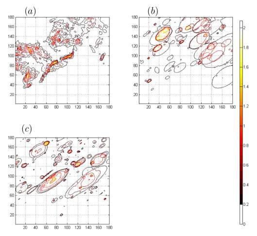
Spatial-temporal rainfall models based on Poisson cluster processes                         3

                                                (b) Spatial maximum rainfall (mm) over time.
 (a) Sample rainfall for a single time point.

                                                (d) Percentage of sample area covered by rain-
 (c) Spatial mean rainfall (mm) over time.
                                                fall over time.

Fig. 1: Rainfall on 24th September 201 from 12:54 to 16:48 hours at Laverton,
Melbourne.

2 The Cox-Isham-Northrop model and extensions

The Cox-Isham-Northrop (CIN) rainfall model is a spatial-temporal stochastic
model for a rainfall event, constructed using a cluster point process. The cluster
process is constructed by taking a primary point process, called the storm
arrival process, and then attaching to each storm center a finite secondary
point process, called a cell process. To each cell center we then attach a rain
cell, with an associated area, duration and intensity. The storm and cell centers
all share a common velocity. The total rainfall intensity at point (x, y) and time
t is then the sum of the intensity at (x, y) of all cells active at time t [6, 10].
   The storm arrival process is taken to be a Poisson process in R2 × [0, ∞)
with homogeneous rate λs . Let v = (vx , vy ) be the velocity of the rainfall
event, so if a storm center arrives at (u, s) then at time s + t it will be at
(u + tv, s + t). Storm durations are random with an exp(γs ) distribution.
   While a storm is active it produces cells at a rate λc in time, starting
with a cell at the moment the storm begins. If the storm arrives at (u, s) and
produces a cell at time s + t, the cell will be centered at u + tv + w, where w
comes from a Gaussian distribution with mean 0 and covariance Σ. The cell
centre then also moves with velocity v. We parameterise Σ using the storm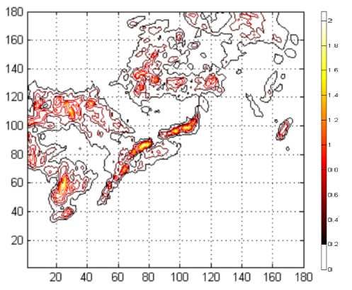
4                                                                         Nanda R. Aryal, Owen D. Jones

           a)    1   1         1               2      2         2     2    2
                S1 S2 − S1                    S1     S2 − S1         S3 − S2

            T1                           T2

           b)

                           D1                                   D2

                                   L12

                                               X12

                                                                               X32
                         L11

                                                          X22
Fig. 2: Schematic of the temporal structure of the CIN model: a) Storm process
(storm origins at Ti ) and cell processes (the solid points show cell origins). The
Sij note the times from the storm origins to cell origins; b) Storm durations
Di , cell durations Lji , and cell intensities Xij .

diameter ds , eccentricity e and orientation ω. d−1
                                                  s  has a gamma distribution
with mean µ1/ds and coefficient of variation CV1/ds .
    Individual cells have random durations, distributed as exp(γc ), and ran-
dom diameters dc (the major axis). Rain cells are elliptical, with the same
eccentricity e and orientation ω as the storms. d−1c has a gamma distribution
with mean µ1/dc and coefficient of variation CV1/dc . It is convenient to use
µA , the expected area of a rain cell, instead of CV1/dc , where
                              p
                       µA = π 1 − e2 µ1/dc (1 + CV1/d−2
                                                       c
                                                         ).

   For the CIN model the intensity of a rain cell is constant over the area
and duration of the cell, with an exponential distribution mean µX . The dis-
placement, duration, diameter, and intensity of a cell are all independent, and
independent of other cells. We give a schematic of the temporal structure of
the CIN model in Figure 2 and of the spatial structure in Figure 3.
   All together the CIN model has 13 parameters: velocity v = (vx , vy ); ec-
centricity e; orientation ω; storm rate λs ; mean storm duration 1/γs ; storm
diameter given by µ1/ds and CV1/ds ; cell rate λc ; mean cell duration 1/γc ; cell
diameter given by µ1/dc and µA ; and mean cell intensity µX .

2.1 Generalisations of the CIN model

We extend the model in two stages. In both cases the temporal structure of
the process is unchanged and we refine the spatial structure of the rain cells.
    The first stage we call the CIN-1 model. With this model we primarily
seek to capture an observed variation in the eccentricity of the cells: some
cells appear circular in shape while some are long and thin. Accordingly we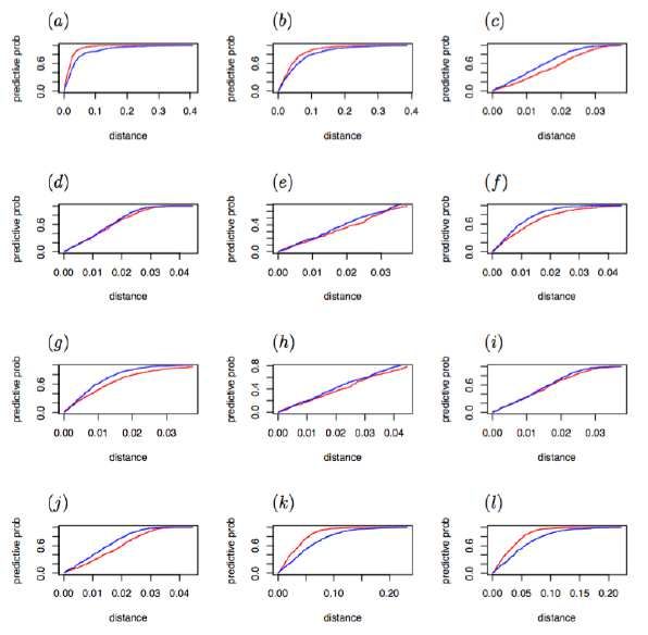
Spatial-temporal rainfall models based on Poisson cluster processes            5

                                                                      ⋆

                             ⋆

                                            ⊗
                                                    ⋆

                                     ⋆

Fig. 3: Schematic diagram of the spatial structure of the CIN model. The
centre point is a storm centre (which has a constant velocity). Stars are cell
centres and the lines indicate the displacement of cell centres from the storm
centre. The dashed curves indicate the cell areas, and the dotted curve gives
a 95% prediction region for the storm area.

suppose that cell eccentricity has a normal distribution with mean µe and
variance σe2 , truncated to [0, 1].
    Also to provide a better match with observations, we suppose that the
rainfall intensity decreases continuously from the centre of a cell to the edge,
rather than acting as a step function. If a and b are the lengths of the semi-
major and semi-minor axis of a rain cell, and X is the intensity at the cell
centre (cx , cy ), then we model the intensity at (x, y) as
                            r
                                    (x − cx )2   (y − cy )2
                          X 1−           2
                                               −            .
                                       a            b2
    For the second stage CIN-2 model we introduce further changes aimed
at making it easier to capture high localised intensities. Specifically, for cell
intensity X and cell diameter dc , we suppose that
                                       2

                 X            µX           σX       ρX,dc σX σdc
            log       ∼N            ,
                 dc           µdc      ρX,dc σX σdc     σd2c

    Figure 4 represents the intensity of a single cell in (a) the CIN model and
(b) the CIN-1 and CIN-2 models.

3 Model Fitting Using ABC

ABC is a likelihood-free Bayesian inference technique, which uses simulations
from the likelihood of interest in the absense of an analytic form. The technique
developed from numerically intensive techniques for estimating population ge-
netics models [13], and has since seen steadily increasing use in a variety of
applications. The recent collection edited by Sisson, Fan and Beaumont [16]
gives a comprehensive introduction to the subject. In what follows we use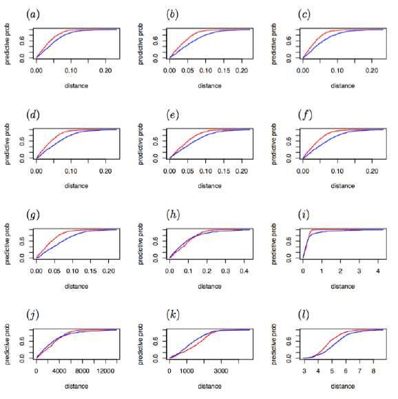
6                                                      Nanda R. Aryal, Owen D. Jones

(a)                                                      (b)

                            X                                              X

                                dc                                               dc

      Fig. 4: Cell intensities for (a) CIN model (b) CIN-1 and CIN-2 models

ABC-MCMC, introduced by Marjoram et al. [8], which uses Markov Chain
Monte Carlo to speed up the effective sampling rate of vanilla ABC.
    We suppose that we have an observation D from some model f (·|θ), de-
pending on parameters θ, and that we are able to simulate from f . Let π
be the prior distribution for θ and S = S(D) a vector of summary statis-
tics for D, then ABC generates samples from f (θ|ρ(S(D∗ ), S(D)) < ǫ), where
D∗ ∼ f (·|θ), θ ∼ π, and ρ is some distance function. If S is a sufficient statistic,
then as ǫ → 0 this will converge to the posterior f (θ|D). ABC-MCMC adds a
proposal chain with density q and an additional rejection step, to generate a
sample {θ i }. The algorithm is as follows:
          FOR i = 1 to N
            1 Given current state θ i propose a new state θ ∗ using q(·|θ i )
            2 Put α = min {1, (π(θ ∗ )q(θ i |θ ∗ ))/(π(θ i )q(θ ∗ |θ i ))}
            3 Go to 4 with probability α, otherwise set θ i+1 = θ i and
             return to 1
            4 Simulate data D∗ ∼ f (·|θ ∗ )
            5 If ρ(S(D∗ ), S(D)) ≤ ǫ then set θ i+1 = θ ∗ , otherwise set
             θ i+1 = θ i
         END FOR
    Unlike [8] we put the MCMC rejection step 3 before the ABC comparison
step 5, to avoid unnecessarily running the simulation in step 4. Note that if
we wish to use a non-uniform kernel in step 5 (see for example Sisson and Yan
[15] §4.3) then we can no longer separate the MCMC rejection step and the
ABC comparison step, which increases the simulation burden. Sisson and Yan
argue that using a kernel with unbounded support can improve the mixing of
the Markov chain, however we did not find this to be a problem. In particular,
using a regression adjustment [3] allows some relaxation of the threshold ǫ, to
increase the acceptance rate without deliteriously impacting the posterior.
    Practically, if θ 0 has very low posterior probability then ABC-MCMC can
fail to accept any new sample points. Previous authors have suggested using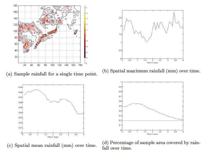
Spatial-temporal rainfall models based on Poisson cluster processes            7

a separate ABC step (without MCMC) to find a θ 0 with large posterior prob-
ability; we found that using Simulated Method of Moments (SMM) instead
requires much less computation time. SMM is a variant of the Generalised
Method of Moments (GMM) that uses Monte-Carlo estimates of moments,
rather than analytic expressions (McFadden 1989 [9]). Thus, like ABC, using
SMM we have much more freedom in the choice of moments used to fit the
model to the data, and we found that it worked well using the same summary
statistics S that we use for the ABC fitting.
    Following Wheater et al. [18], for the CIN model the velocity v, eccentricity
e and orientation ω were all estimated using temporal and spatial autocovari-
ance estimates, and then fixed. For the CIN-1 and CIN-2 models we used our
estimate of e for µe but also need to estimate σe2 . To do this we divided the
study region spatially into four equal parts, then estimated the eccentricity
for each part at each time point, giving four time-series of estimates for µe .
Treating each series as an AR(1) process with mean µe , we can correct for the
autocorrelation to get the usual moment-based estimate for σe2 .
    The remaining parameters are all estimated using ABC. We used the same
set of 23 summary statistics for the CIN, CIN-1, and CIN-2 models:
 – The overall mean and standard deviation of rainfall, taken over all pixels
   and all times.
 – The spatial-temporal auto-correlation, with lags of (x, y, t), where x and y
   are measured in pixels and t is in units of 6-minutes. We take t = 0, x ∈
   {−1, 0, 1}, y ∈ {−1, 0, 1}, and t = 1, x ∈ {−1, 0, 1}+vx , y ∈ {−1, 0, 1}+vy .
   Here vx and vy are the velocity components, in units of pixels per 6-minutes.
   Note that the lag (0, 0, 0) auto-correlation is just the variance and so has
   already been included.
 – The probability of an arbitrary pixel and time being dry.
 – The ratio of dry/wet area and mean and standard deviation of wet area,
   averaged over time.

P For the     distance function ρ we used a weighted sum of squares ρ(S(D∗ ), S(D)) =
    w
   i i (S ∗
            (i) − S(i))2 , where S ∗ (i) and S(i) are the i-th components of S(D∗ )
and S(D) respectively. We found empirically that a good choice for wi is to
take it inversely proportional to the variance of S ∗ (i) conditioned on using a θ
with high posterior probability. Given that θ 0 was chosen using SMM to have
maximal posterior probability, we used a separate sample of S(D∗ ) given θ 0
to estimate the wi .
    The choice of summary statistics S and distance metric ρ plays a large
part in the performance of ABC. Ideally S should be sufficient, but certainly
it should reflect those aspects of the real process considered most important.
However choosing S too large reduces the efficiency of ABC, though this can
be mitigated to some extent by using a regression adjustment, for which we
used the approach of Beaumont et al. [3].
    The remaining parameters were transformed to reduce dependence and
skewness, and mapped to (−∞, ∞). This makes it easier for the proposal
chain to spend its time in regions of high posterior probability. Vague normal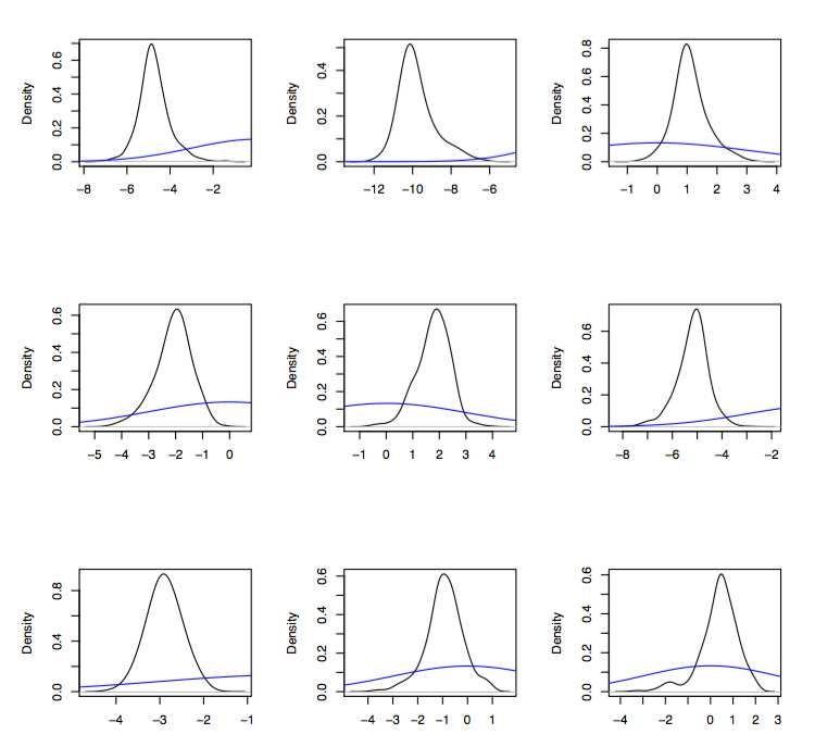
8                                                   Nanda R. Aryal, Owen D. Jones

priors are used for all the transformed parameters, and for the proposal chain
we used a random walk with N (0, 0.22 I) steps.
    For the CIN and CIN-1 model our new ABC-parameters are

             θ(1) = log(λs γs−1 ),             θ(2) = log(λs γs ),
             θ(3) =   log(λc γc−1 ),           θ(4) = log(λc γc ),
             θ(5) = log(µX µA ),               θ(6) = log(µX µ−1
                                                              A ),
             θ(7) = log(µ1/dc ),               θ(8) = log(µ1/ds ),
             θ(9) = log(CV1/ds ),

   For the CIN-2 model we replace parameters µ1/dc and µA by µdc and σd2c ,
                     2
and gain parameters σX and ρX,dc .

            ψ(1) = log(λs γs−1 ),                  ψ(2) = log(λs γs ),
            ψ(3) =   log(λc γc−1 ),                ψ(4) = log(λc γc ),
                                                                 2
            ψ(5) = log(µX ),                       ψ(6) = log(1/σX ),
            ψ(7) = log(µdc ),                      ψ(8) = log(1/σd2c ),

                         ρX,dc + 1
            ψ(9) = log               ,            ψ(10) = log(µ1/ds ),
                         1 − ρX,dc
           ψ(11) = log(CV1/ds )

3.1 Comparison of Fitted Models

Using the spatial autocorrelation function we estimated v = (vx , vy ) = (0.10, 29.9),
e = µe = 0.86, σe2 = 0.04 and ω = 39◦ .
     In the appendix Figures 10–12 plot the posterior sample traces for models
CIN, CIN-1 and CIN-2. In each case the chains appear stationary and exhibit
good mixing.
     For the CIN model using a threshold of ǫ = 10 the overall acceptance
rate was approximately 4.1%. Increasing ǫ improves the acceptance rate and
the degree of mixing, at the expense of reduced accuracy for the posterior
approximation. For the CIN-1 and CIN-2 models the acceptance rates were
approximately 5% and 11% respectively, using thresholds of ǫ = 14 and 8. For
ABC-MCMC rather than the acceptance rate, a better measure of sampling
efficiency is the “effective sample rate” for each parameter. That is, the effec-
tive sample size over number of simulations required to produce them. For the
CIN, the effective sample rate varied from 0.002 to 0.004 depending on the
parameter. For the CIN1 and CIN2 models the effective sample rate varied
from 0.001 to 0.003 and from 0.001 to 0.005 respectively.
     Posterior plots for models CIN, CIN-1 and CIN-2 are given in Figures 5–7.
In all three cases we get nice peaks on our posteriors.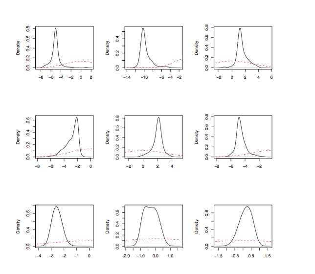
Spatial-temporal rainfall models based on Poisson cluster processes              9

Fig. 5: CIN model: posteriors for θ(i), i = 1, 2, ..., 9. Priors are given by the
dashed lines.

Fig. 6: CIN-1 model: posteriors for θ(i), i = 1, 2, ..., 9. Priors are given by the
dashed lines.
10                                                                                                                  Nanda R. Aryal, Owen D. Jones

                 0.0 0.4 0.8
       Density

                                                                        Density

                                                                                                                    Density

                                                                                                                              0.6
                                                                                  0.4
                                                                                  0.0

                                                                                                                              0.0
                                     −8       −6   −4      −2                           −16    −12      −8 −6                       −4    −2       0        2   4
       Density

                                                                        Density

                                                                                                                    Density

                                                                                                                              0.6
                 0.6

                                                                                  0.4
                 0.0

                                                                                  0.0

                                                                                                                              0.0
                                     −8       −6   −4          −2                        −5     −3     −1 0     1                   −2         0        2       4
                                                                                  0.8
       Density

                                                                        Density

                                                                                                                    Density
                 0.6

                                                                                                                              0.4
                                                                                  0.4
                 0.0

                                                                                  0.0

                               −2        −1   0    1       2        3                   −1.5   −0.5   0.5     1.5             0.0    −6    −4      −2       0   2   4
       Density

                                                                        Density
                 0.6

                                                                                  0.6
                 0.0

                                                                                  0.0

                                    −4        −2       0   1    2                       −1.5   −0.5   0.5     1.5

Fig. 7: CIN-2 model: posteriors for ψ(i), i = 1, 2, ..., 11. Priors are given by the
dashed lines.

    Posterior summaries for the original parameters are given in Tables 1–3 in
the Appendix. The fitted CIN-2 model shows moderate evidence of negative
correlation between cell intensity and diameter: the posterior mean for ρX,dc
is −0.69 with a 95% credible interval of (−0.93, 0.10).
    To compare the performance of our three models we use posterior predictive
probabilities to judge how close each model is to the original data, as measured
by our distance ρ. That is, we compare for each model the distribution of
ρ(S(D∗ ), S(D)) where D is the original data and D∗ is generated by the model
when θ is distributed according to the posterior. We can sample from this
distribution by sampling θ from the posterior, generating D∗ from θ and the
model, and then calculating ρ(S(D∗ ), S(D)). We can then estimate the c.d.f.
of ρ(S(D∗ ), S(D)) using the e.d.f. of a suitably large sample.
  Figure 8 plots the estimated c.d.f. of the posterior for ρ(S(D∗ ), S(D)) under
models CIN and CIN-1. We see that under CIN-1 smaller distances are more
Spatial-temporal rainfall models based on Poisson cluster processes 11
total distance
predictive prob
0.6
0.0
3 4 5 6 7 8
distance
Fig. 8: Posterior distribution of ρ(S(D∗ ), S(D)) for the CIN model (blue) and
CIN-1 model (red). The CIN-1 model is more likely to produce simulations
D∗ close to D, as measured by ρ.
likely, that is the fitted CIN-1 model is more likely to produce data closer to
our observation.
We can also construct posterior predictive distributions for (S ∗ (i) − S(i))2 .
That is, we can compare the fit of each model as measured by individual
components of the summary statistic S. They are given in Figures 13 and
14 in the Appendix. Generally the CIN-1 model performs better, though not
uniformly, but without any obvious pattern to the exceptions.
Quantitatively the CIN-1 model is an improvement over the CIN model.
We can also see this qualitatively with some sample plots. In Figure 9 we give
sample contour plot of the spatial rainfall intensity at a single time-point for
(a) the data; (b) the fitted CIN model; and (c) the fitted CIN-1 model.
Acknowledgements Datasets for this research are available from the Australian Bureau of
Meteorology, GPO Box 1289, Melbourne VIC 3001. http://www.bom.gov.au/climate/data-
services/data-requests.shtml. The Bureau charges according to the Australian Government
Cost Recovery Guidelines.12 Nanda R. Aryal, Owen D. Jones Fig. 9: (a) Calibrated rainfall radar data, courtesy of the Australian Bureau of Meteorology. (b) A simulation from the fitted CIN model. (c) A simulation from the fitted CIN-1 model. Appendix Fig. 10: ABC-MCMC fitting for CIN model: posterior chains for θ(i), i = 1, 2, . . . , 9.
Spatial-temporal rainfall models based on Poisson cluster processes    13

Fig. 11: ABC-MCMC fitting for CIN-1 model: posterior chains for θ(i), i =
1, 2, . . . , 9.
14                                                   Nanda R. Aryal, Owen D. Jones

Fig. 12: ABC-MCMC fitting for CIN-2 model: posterior chains for ψ(i),i =
1, 2, . . . , 11.

               Parameter     Mean    Median    95 % Credible Interval
                   λs       0.0008    0.0006         (0.0003, 0.0026)
                  γs−1     14.8159   13.2333        (2.9086, 38.5852)
                   λc       0.6968    0.6201         (0.2321, 1.7451)
                  γc−1      5.3733    4.6462        (2.6768, 13.1802)
                 µ1/ds      0.5199    0.4006         (0.0738, 1.8749)
                CV1/ds      1.9438    1.5953         (0.1467, 6.0694)
                  µX        0.1946    0.1917         (0.0792, 0.3332)
                  µA       37.2997   32.6773       (11.8394, 93.7327)
                 µ1/dc      0.0595    0.0548         (0.0255, 0.1211)

     Table 1: Posterior estimates of the ABC-parameters for the CIN model.
Spatial-temporal rainfall models based on Poisson cluster processes 15
Parameter Mean Median 95 % Credible Interval
λs 0.0008 0.0005 (0.0002 0.0036)
γs−1 12.7340 12.3910 (1.0938 38.4967)
λc 0.6166 0.5722 (0.1171, 1.8787)
γc−1 10.7880 7.6703 (4.0369, 35.9604)
µ1/ds 0.8022 0.7224 (0.3761, 1.6064)
CV1/ds 1.2535 1.2105 (0.5601, 2.1132)
µX 0.2850 0.2731 (0.1508, 0.4848)
µA 33.0017 31.5407 (4.6533, 92.1609)
µ1/dc 0.0840 0.0771 (0.0441, 0.1617)
Table 2: Posterior estimates of the ABC-parameters for the CIN-1 model.
Parameter Mean Median 95% Credible Interval
λs 0.0006 0.0006 (0.0002, 0.00150
γs−1 31.797 32.462 (4.4944, 64.524)
λc 0.1887 0.1801 (0.0457, 0.4429)
γc−1 13.883 11.407 (5.6338, 42.133)
µ1/ds 1.3331 1.1647 (0.1671, 4.3280)
CV1/ds 1.2102 1.1901 (0.6291, 1.9917)
µX 0.1882 0.1258 (0.0426, 0.7603)
σX2 0.5235 0.4519 (0.0671, 1.5503)
µd c 2.7478 2.7523 (0.7829 , 5.6306)
σd2c 0.8602 0.7859 (0.4335, 1.7103)
ρX,dc -0.6906 -0.7564 (-0.9327, 0.0996)
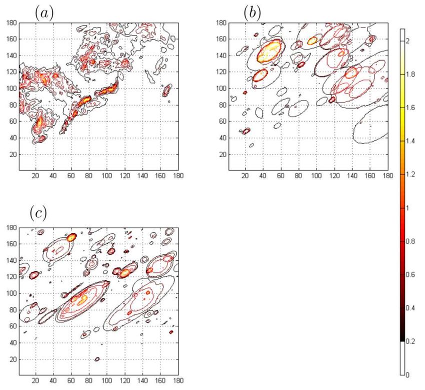
Table 3: Posterior estimates of the ABC-parameters for the CIN-2 model.16 Nanda R. Aryal, Owen D. Jones Fig. 13: Predictive probability for the CIN model (blue line) and CIN-1 model (red line). Plots (a) and (b) are for mean and stan- dard deviation summaries. Plots (c) to (j) are spatial correlations ρ(−1, −1, 0), ρ(−1, 0, 0), ρ(1, 1, 0), ρ(0, −1, 0), ρ(0, 1, 0), ρ(1, −1, 0), ρ(1, 0, 0), and ρ(1, 1, 0). Plots (k) and (l) are of ρ(−1 + vx , −1 + vy , 1), and ρ(−1 + vx , 0 + vy , 1).
Spatial-temporal rainfall models based on Poisson cluster processes 17
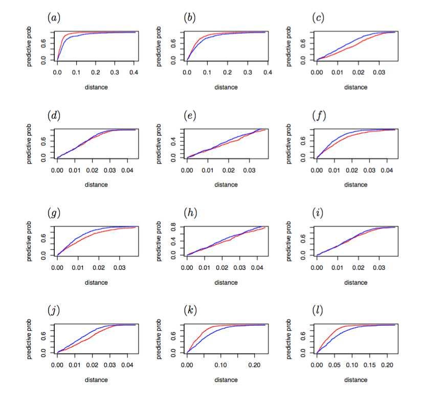
Fig. 14: Predictive probability for the CIN model (blue line) and CIN-1 model
(red line). Plots (a) to (g) are of spatial autocorrelations ρ(−1 + vx , 1 +
vy , 1), ρ(0+vx , −1+vy , 1), ρ(0+vx , 0+vy , 1), ρ(0+vx , 1+vy , 1), ρ(1, +vx , −1+
vy , 1), ρ(1, +vx , 0 + vy , 1), and ρ(1, +vx , 1 + vy , 1). Plots (h) and (i) are of dry
probability of an arbitrary pixel and dry and wet area ratio. Plots (j) and (k)
are of mean wet area over time and standard deviation of wet area over time.
Plot (l) is of total distance form all summaries.
References
1. Aryal, N.R.: Stochastic spatial-temporal models for rainfall processes. Ph.D. thesis,
School of Mathematics and Statistics, The University of Melbourne (2018)
2. Aryal, N.R., Jones, O.D.: Fitting the Bartlett–Lewis rainfall model using Approximate
Bayesian Computation. Mathematics and Computers in Simulation (2019)
3. Beaumont, M.A., Zhang, W., Balding, D.J.: Approximate Bayesian Computation in
population genetics. Genetics 162(4), 2025–2035 (2002)18 Nanda R. Aryal, Owen D. Jones
4. Benoit, L., Allard, D., Mariethoz, G.: Stochastic rainfall modeling at sub-kilometer
scale. Water Resources Research 54(6), 4108–4130 (2018)
5. Chandler, R., Isham, V., Northrop, P., Wheater, H., Onof, C., Leith, N.: Uncertainty in
rainfall inputs. Applied Uncertainty Analysis for Flood Risk Management, edited by:
Beven, KJ and Hall, JW, Imperial College Press: London pp. 101–152 (2014)
6. Cox, D.R., Isham, V.: A simple spatial-temporal model of rainfall. Proceedings of the
Royal Society of London. A. Mathematical and Physical Sciences 415(1849), 317–328
(1988)
7. Jones, O.D., Nyman, P., Sheridan, G.J.: Modelling the effects of fire and rainfall regimes
on extreme erosion events in forested landscapes. Stochastic Environmental Research
and Risk Assessment 28(8), 2015–2025 (2014)
8. Marjoram, P., Molitor, J., Plagnol, V., Tavaré, S.: Markov chain monte carlo without
likelihoods. Proceedings of the National Academy of Sciences 100(26), 15324–15328
(2003)
9. McFadden, D.: A method of simulated moments for estimation of discrete response mod-
els without numerical integration. Econometrica: Journal of the Econometric Society
pp. 995–1026 (1989)
10. Northrop, P.: A clustered spatial-temporal model of rainfall. Proceedings of the
Royal Society of London. Series A: Mathematical, Physical and Engineering Sciences
454(1975), 1875–1888 (1998)
11. Onof, C., Chandler, R., Kakou, A., Northrop, P., Wheater, H., Isham, V.: Rainfall
modelling using poisson-cluster processes: a review of developments. Stochastic Envi-
ronmental Research and Risk Assessment 14(6), 384–411 (2000)
12. Paschalis, A., Molnar, P., Fatichi, S., Burlando, P.: A stochastic model for high-
resolution space-time precipitation simulation. Water Resources Research 49(12), 8400–
8417 (2013)
13. Pritchard, J.K., Seielstad, M.T., Perez-Lezaun, A., Feldman, M.W.: Population growth
of human y chromosomes: a study of y chromosome microsatellites. Molecular biology
and evolution 16(12), 1791–1798 (1999)
14. Segond, M.L., Wheater, H.S., Onof, C.: The significance of spatial rainfall representation
for flood runoff estimation: A numerical evaluation based on the Lee catchment, UK.
Journal of Hydrology 347(1-2), 116–131 (2007)
15. Sisson, S., Fan, Y.: ABC samplers. In: Handbook of Approximate Bayesian Computa-
tion, pp. 87–123. Chapman and Hall/CRC (2018)
16. Sisson, S.A., Fan, Y., Beaumont, M. (eds.): Handbook of Approximate Bayesian Com-
putation. Handbooks of Modern Statistical Methods. CRC Press (2018)
17. Wheater, H., Chandler, R., Onof, C., Isham, V., Bellone, E., Yang, C., Lekkas, D.,
Lourmas, G., Segond, M.L.: Spatial-temporal rainfall modelling for flood risk estimation.
Stochastic Environmental Research and Risk Assessment 19(6), 403–416 (2005)
18. Wheater, H., Isham, V., Chandler, R., Onof, C., Stewart, E.: Improved methods for
national spatial-temporal rainfall and evaporation modelling for BSM (2006)Figures Figure 1 See the Manuscript Files section for the complete gure caption.
Figure 2

See the Manuscript Files section for the complete gure caption.

Figure 3

See the Manuscript Files section for the complete gure caption.

Figure 4

See the Manuscript Files section for the complete gure caption.
Figure 5

See the Manuscript Files section for the complete gure caption.
Figure 6

See the Manuscript Files section for the complete gure caption.

Figure 7

See the Manuscript Files section for the complete gure caption.
Figure 8

See the Manuscript Files section for the complete gure caption.

Figure 9

See the Manuscript Files section for the complete gure caption.
Figure 10

See the Manuscript Files section for the complete gure caption.
Figure 11

See the Manuscript Files section for the complete gure caption.
Figure 12

See the Manuscript Files section for the complete gure caption.
Figure 13

See the Manuscript Files section for the complete gure caption.
Figure 14

See the Manuscript Files section for the complete gure caption.
You can also read