Retinal OCT Denoising with Pseudo-Multimodal Fusion Network
←
→
Page content transcription
If your browser does not render page correctly, please read the page content below
Retinal OCT Denoising with
                                                       Pseudo-Multimodal Fusion Network

                                          Dewei Hu1 , Joseph D. Malone2 , Yigit Atay1 , Yuankai K. Tao2 , and Ipek Oguz1
                                              1
                                                  Vanderbilt University, Dept. of Electrical Engineering and Computer Science,
                                                                             Nashville, TN, USA
                                              2
                                                  Vanderbilt University, Dept. of Biomedical Engineering, Nashville, TN, USA
arXiv:2107.04288v1 [eess.IV] 9 Jul 2021

                                                   Abstract. Optical coherence tomography (OCT) is a prevalent imag-
                                                   ing technique for retina. However, it is affected by multiplicative speckle
                                                   noise that can degrade the visibility of essential anatomical structures,
                                                   including blood vessels and tissue layers. Although averaging repeated
                                                   B-scan frames can significantly improve the signal-to-noise-ratio (SNR),
                                                   this requires longer acquisition time, which can introduce motion ar-
                                                   tifacts and cause discomfort to patients. In this study, we propose a
                                                   learning-based method that exploits information from the single-frame
                                                   noisy B-scan and a pseudo-modality that is created with the aid of the
                                                   self-fusion method. The pseudo-modality provides good SNR for layers
                                                   that are barely perceptible in the noisy B-scan but can over-smooth fine
                                                   features such as small vessels. By using a fusion network, desired features
                                                   from each modality can be combined, and the weight of their contribu-
                                                   tion is adjustable. Evaluated by intensity-based and structural metrics,
                                                   the result shows that our method can effectively suppress the speckle
                                                   noise and enhance the contrast between retina layers while the overall
                                                   structure and small blood vessels are preserved. Compared to the single
                                                   modality network, our method improves the structural similarity with
                                                   low noise B-scan from 0.559 ± 0.033 to 0.576 ± 0.031.

                                                   Keywords: Optical coherence tomography · denoising · self-fusion.

                                          1       Introduction
                                          Optical coherence tomography (OCT) is a powerful non-invasive ophthalmic
                                          imaging tool [9]. The limited light bandwidth of the imaging technique on which
                                          OCT is based upon, low-coherence interferometry [15], gives rise to speckle noise
                                          that can significantly degrade the image quality. In clinical practice, the thick-
                                          ness of the retina layers, such as the ganglion cell layer (GCL), inner plexiform
                                          layer (IPL) and retinal nerve fiber layer (RNFL), are of interest [16]. Retinal
                                          OCTs also reveal the vascular system, which is important for ocular diseases like
                                          diabetic retinopathy [12]. The speckle noise in single frame B-scans makes the
                                          border of layers unclear so that it is hard to distinguish adjacent layers, such as
                                          the GCL and IPL. The noise also produces bright dots and dark holes that can
                                          hurt the homogeneity of layers and affect the visibility of the small vessels within
                                          them. A proper denoising method is thus paramount for ophthalmic diagnosis.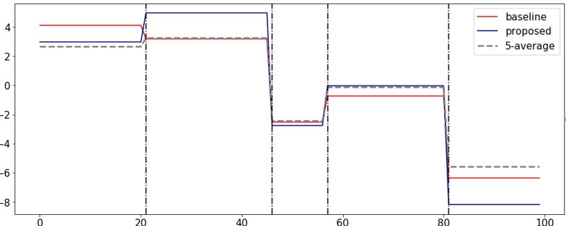
2         D. Hu et al.

    Acquiring multiple frames at the same anatomical location and averaging
these repeated frames is the mainstream technique for OCT denoising. The more
repeated frames are acquired, the closer their mean can be to the ideal ground
truth. However, this increases the imaging time linearly, and can cause discomfort
to patients as well as increase motion artifacts. Other hardware-based OCT
denoising methods including spatial [1] and angular averaging [14] will similarly
prolong the acquisition process. Ideally, an image post-processing algorithm that
applies to a single frame B-scan is preferable. Throughout the paper, we denote
single frame B-scan as high noise (HN) and frame-average image as low noise
(LN).
    The multiplicative nature of speckle noise makes it hard to be statistically
modelled, as the variation of noise intensity level in different tissue increases
the complexity of the problem [4]. In a recent study, Oguz et al. [11] proposed
the self-fusion method for retinal OCT denoising. Inspired by multi-atlas label
fusion [17], self-fusion exploits the similarity between adjacent B-scans. For each
B-scan, neighboring slices within radius r are considered as ‘atlases’ and vote
for the denoised output. As shown in Fig. 1, self-fusion works particularly well
in preserving layers, and in some cases it also offers compensation in vessels.
However it suffers from long computation time and loss of fine details, similar to
block-matching 3D (BM3D) [5] and k singular value decomposition (K-SVD) [8].
    Deep learning has become the state-of-the-art in many image processing tasks
and shown great potential for image noise reduction. Although originally used
for semantic segmentation, the U-Net [13] architecture enables almost all kinds
of image-to-image translation [7]. Formulated as the mapping of a high noise
image to its ‘clean’ version, the image denoising problem can easily be seen as
a supervised learning algorithm. Because of the poor quality of single frame B-
scan, more supplementary information and constraints are likely to be beneficial
for feature preservation. For instance, observing the layered structure of the
retina, Ma et al. [10] introduce an edge loss function to preserve the prevailing
horizontal edges. Devalla et al. [6] investigate a variation to U-Net architecture
so that the edge information is enhanced.
    In this study, we propose a novel despeckling pipeline that takes advantage of
both self-fusion and deep neural networks. To boost the computational efficiency,
we substitute self-fusion with a network that maps HN images to self-fusion
of LN, which we call a ‘pseudo-modality’. From this smooth modality, we can
easily extract a robust edge map to serve as a prior instead of a loss function.
To combine the useful features from different modalities, we introduce a pseudo-
multimodal fusion network (PMFN). It serves as a blender that can ‘inpaint’ [3]
the fine details from HN on the canvas of clean layers from the pseudo-modality.
The contributions of our work are the following:

     A deep network to mimic the self-fusion process, so that the self-fusion of
      LN image becomes accessible at test time. This further allows the processing
      time to be sharply reduced.
OCT Denoising with PMFN 3
High-noise (HN) Low-noise (LN) Self-fusion of HN Self-fusion of LN
ONH
Fovea
Fig. 1. Self-fusion for high-noise (HN) single B-scan and low-noise (LN) 5-average
images (excess background trimmed). SNR of the HN images is 101dB.
Fig. 2. Processing pipeline. Dotted box refers to a deep learning network. Process on
dash arrow exists only in training. Solid arrows are for both training and testing.
A pseudo-modality that makes it possible to extract clean gradient maps
from high noise B-scans and provide compensation of layers and vessels in
the final denoising result.
A pseudo-multimodal fusion network that combines desired features from
different sources such that the contribution of each modality is adjustable.
2 Methods
Fig. 2 illustrates the overall processing pipeline.
Preprocessing. We crop every B-scan to size [512, 500] to discard the mas-
sive background that is not of interest. Then we zero-pad the image to [512, 512]
for convenience in downsampling.4 D. Hu et al.
5-frame average. In our supervised learning problem, the ground truth
is approximated by the low noise 5-frame-average B-scan (LN). The repeated
frames at location i are denoted by [Xi1 , ..., Xi5 ] in Fig. 2-a. Because of eye
movement during imaging, some drifting exists between both repeated frames
and adjacent B-scans. We apply a rigid registration for motion correction prior
to averaging.
Pseudo-modality creation. For self-fusion, we need deformable registra-
tion between adjacent slices. This is realized by VoxelMorph [2], a deep registra-
tion method that provides deformation field from moving image to target. This
provides considerable speedup compared to traditional registration algorithms.
However, even without classical registration, self-fusion is still time-consuming.
To further reduce the processing time, we introduce Network 1 to directly learn
the self-fusion output. Time consumed by generating a self-fusion image of a
B-scan drops from 7.303 ± 0.322s to 0.253 ± 0.005s. The idea allows us to also
improve the quality of our pseudo-modality, by using Si , the self-fusion of LN
Yi images rather than that of HN images. Thus, Network I maps a stack of
consecutive HN B-scans to self-fusion of LN.
In Fig. 2-b, the noisy B-scan and its neighbors within a radius are denoted
j j
as [Xi−r , ..., Xi+r ], where j = 1, 2, . . . , 5 represent the repeated frames. Their
corresponding LN counterparts are named similarly, [Yi−r , ..., Yi+r ]. The ground
truth of Network I (i.e., the self-fusion of Yi ) and its prediction are annotated
j j
as Si and S̃i respectively. Since S̃i contains little noise, we can use its image
gradient Gji , computed simply via 3x3 Sobel kernels, as the edge map.
Psudo-multimodal fusion network (PMFN). Fig. 2-c shows the PMFN
that takes a three-channel input. The noisy B-scan Xij has fine details including
small vessels and texture, while the speckle noise is too strong to clearly reveal
j
layer structures. The pseudo-modality S̃i has well-suppressed speckle noise and
clean layers, but many of the subtle features are lost. So, merging the essential
features from these mutually complementary modalities is our goal. To produce
an output that inherit features from two sources, Network II takes feedback from
the ground truth of both modalities in seeking for a balance between them. We
use L1 loss for Yi to punish loss of finer features and mean squared error (MSE)
for Si to encourage some blur effect in layers. The weight of these loss functions
are determined by hyper-parameters. The overall loss function is:
X j β X j
Loss = α |Ỹi (x, y) − Yi (x, y)| + (Ỹi (x, y) − Si (x, y))2 (1)
x,y
N x,y
N is the number of pixel in the image. Parameters α and β are the weights of
the two loss functions, and they can be tuned to reach a tradeoff between layers
from the pseudo-modality and the small vessels from the HN B-scan.OCT Denoising with PMFN 5 Fig. 3. Network architecture. The solid line passes the computation result of the block while the dash line refers to channel concatenation. Arrays in main trunk blocks indicate the output dimension. 3 Experiments 3.1 Data set OCT volumes from the fovea and optic nerve head (ONH) of a single human retina were obtained. For each region, we have two volumes acquired at three dif- ferent noise levels (SNR=92dB, 96dB, 101dB). Each raw volume ([NBscan , H, W ] = [500, 1024, 500]) contains 500 B-scans of 1024×500 voxels. For every B-scan, there are 5 repeated frames taken at the same position (2500 Bscans in total) so that a 5-frame-average can be used as low-noise ‘ground truth’. Since all these volumes are acquired from a single eye, to avoid information leakage, we denoise fovea volumes by training on ONH data, and vice versa. 3.2 Experimental design In this study, our goal is to show that the denoising result is improved by the processing pipeline that introduces the pseudo-modality. Thus, we will not fo- cus on varying the network structure for better performance. Instead, we will use the Network II with single channel input Xij as the baseline. For this base- line, the loss function will only have feedback from Yi . We hypothesize that the relative results between single modality and pseudo-multimodal denoising will have a similar pattern for other architectures for Network II, but exploring this is beyond the scope of the current study. Since the network architecture is not
6 D. Hu et al.
LN MSUN PMFN
SNR=92dB
SNR=96dB
SNR=101dB
Fig. 4. Fovea denoising results for different input SNR. (Excess background trimmed.)
the focus of our study, we use the same multi-scale U-Net (MSUN) architecture,
shown in Fig. 3 and proposed by Devalla et al. [6], for both Networks I and II.
The B-scan neighborhood radius for self-fusion was set at r = 7. Among the
five repeated frames at each location, we only use the first one (Xi1 ), except
when computing the 5-average Yi . All the models are trained on NVIDIA RTX
2080TI 11GB GPU for 15 epochs with batch size of 1. Parameters in network
are optimized by Adam optimizer with starting learning rate 10−4 and a decay
factor of 0.3 for every epoch. In Network II, we use α = 1 and β = 1.2.
4 Results
4.1 Visual Analysis
We first analyze the layer separation and vessel visibility in the denoised results.
Fig. 4 displays the denoising performance of the proposed algorithm for dif-
ferent input SNR levels. Compared to the baseline model, we observe that PMFN
has better separation between GCL and IPL, which enables the vessels in GCL
to better stand out from noise. Moreover, the improvement of smoothness and
homogeneity in outer plexiform layer (OPL) makes it look more solid and its bor-
der more continuous. In addition, the retinal pigment epithelium (RPE) appears
to be more crisp.
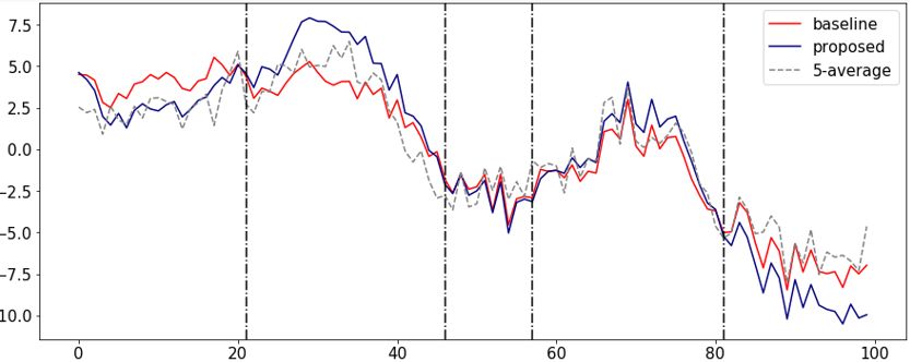
In Fig. 5, to better assess the layer separation, we focus on a B-scan with high
speckle noise (SNR=92) that severely obscures the boundary between layers. InOCT Denoising with PMFN 7
(a) LN (b) MSUN (c) PMFN
(d) Mean column intensity (e) Mean layer intensity
Fig. 5. Layer separation analysis. The top row shows an ROI containing 5 layers of
tissue (GCL, IPL, INL, OPL, ONL) for each of (a) 5-average LN image, (b) baseline
result and (c) PMFN result. (d) plots the intensity across the 5 layers within the
ROI. (e) plots the mean intensity per layer. Vertical dashed lines approximate layer
boundaries.
the top row, we zoom into a region of interest (ROI) that contains 5 tissue layers
(from top to bottom): GCL, IPL, inner nuclear layer (INL), OPL and outer
nuclear layer (ONL). As the baseline model learns only from the high noise B-
scan, layer boundaries are not clear: GCL and IPL are indistinguishable, and
although the INL and OPL are preserved, they are not as homogeneous as in
the PMFN result. PMFN remedies these problems.
Another way of assessing the separability of layers or, in other words, the
contrast between adjacent layers, is plotting the column intensity (Fig. 5-d).
Since the layers within the ROI are approximately flat, we take the mean vector
along the row. In order to rule out the potential difference of intensity level, we
normalize the mean vector with the average intensity of ROI.
W
1 X
v̄ = vi − µROI (2)
W i
where W is the width of the ROI, vi is a column vector in the window and
µROI is a vector that has the mean of the ROI as all its elements. We plot
the v̄ for Fig. 5-a, Fig. 5-b and Fig. 5-c in Fig. 5-d. The border between layers
are approximated with vertical dash lines for this visualization. In Fig. 5-d, the
proposed method tends to have lower intensity in dark bands and higher inten-
sity in bright ones. This indicates that it has better contrast between adjacent
layers. Fig. 5-e summarizes the mean intensity within each layer. Because of8 D. Hu et al.
high intensity speckle noise, the baseline result completely misses the GCL-IPL
distinction, whereas our method provides good separation.
4.2 Quantitative evaluation
We report the signal-to-noise ratio (SNR), peak signal-to-noise ratio (PSNR),
contrast-to-noise ratio (CNR) and structural similarity (SSIM) of our results.
Normally, these metrics need an ideal ground truth without noise as a refer-
ence image. But such a ground truth is not available in our task, since the
5-frame-average LN image is far from being noiseless. Therefore, we make some
adjustments
to the original
definitions of SNR and PSNR. We use SN R =
[f (x,y)]2
P
10 log10 Px,y 2 where f (x, y) is the pixel intensity in foreground win-
x,y [b(x,y)]
dow and b(x, y) is background pixel intensity. This assumes there is nothing
but pure speckle noise in the background, and that the foreground window
only contains signal. Similarly, the PSNR can be approximated by P SN R =
n n max[f (x,y)]2
h i
10 log10 xPy [b(x,y)]2 . The nx and ny are the width and height of the ROI,
x,y
|µ −µ |
respectively. Finally, the CNR is estimated by CN R = √ f 2 b where µf
0.5(σf +σb2 )
and σf are the mean and standard deviation of the foreground region; µb and
σb are those of the background region.
Every layer has a different intensity level, so we report each metric separately
for RNFL, IPL, OPL and RPE. We manually picked foreground and background
ROIs from each layer, as shown in Fig. 6, for 10 B-scans. To avoid local bias,
these chosen slices are far apart to be representative of the whole volume. When
computing metrics for a given layer, the background ROI (yellow box) is cropped
as needed to match the area of the foreground ROI (red box) for that layer. Fig. 7
(a) to (c) display the evaluation result for SNR, PSNR and CNR respectively.
For all layers, the proposed PMFN model gives the best SNR and CNR results,
while the PSNR stays similar with the baseline multi-scale UNet model.
We also report the structural similarity index measure (SSIM) [18] of the
whole B-scan. The SSIM for each input SNR level is reported in Fig. 7-d. The
proposed method outperforms the baseline model for all input SNR.
Fig. 6. Sample B-scans showing background (yellow) and foreground (red) ROIs used
for SNR, CNR and PSNR estimation. 10 B-scans are chosen throughout the fovea
volume to avoid bias.OCT Denoising with PMFN 9
(a) SNR of each layer (b) PSNR of each layer
(c) CNR of each layer (d) SSIM for input of different noise level
Fig. 7. Quantitative evaluation of denoising results.
5 Conclusion and future work
Our study shows that the self-fusion pseudo-modality can provide major contri-
butions to OCT denoising by emphasizing tissue layers in the retina. The fusion
network allows the vessels, texture and other fine details to be preserved while
enhancing the layers. Although the inherent high dimensionality of the deep
network has sufficient complexity, more constraints in the form of additional
information channels are able to help the model converge to a desired domain.
It is difficult to thoroughly evaluate denoising results when no ideal reference
image is available. Exploring other evaluation methods remains as future work.
Additionally, application of our method to other medical image modalities such
as ultrasound images is also a possible future research direction.
Acknowledgements. This work is supported by Vanderbilt University Discov-
ery Grant Program.
References
1. Avanaki, M.R., Cernat, R., Tadrous, P.J., Tatla, T., Podoleanu, A.G., Hojja-
toleslami, S.A.: Spatial compounding algorithm for speckle reduction of dynamic
focus oct images. IEEE Photonics Technology Letters 25(15), 1439–1442 (2013)10 D. Hu et al.
2. Balakrishnan, G., Zhao, A., Sabuncu, M.R., Guttag, J., Dalca, A.V.: Voxelmorph:
a learning framework for deformable medical image registration. IEEE transactions
on medical imaging 38(8), 1788–1800 (2019)
3. Bertalmio, M., Sapiro, G., Caselles, V., Ballester, C.: Image inpainting. In: Pro-
ceedings of the 27th annual conference on Computer graphics and interactive tech-
niques. pp. 417–424 (2000)
4. Chen, Z., Zeng, Z., Shen, H., Zheng, X., Dai, P., Ouyang, P.: Dn-gan: Denoising
generative adversarial networks for speckle noise reduction in optical coherence
tomography images. Biomedical Signal Processing and Control 55, 101632 (2020)
5. Chong, B., Zhu, Y.K.: Speckle reduction in optical coherence tomography images
of human finger skin by wavelet modified bm3d filter. Optics Communications 291,
461–469 (2013)
6. Devalla, S.K., Subramanian, G., Pham, T.H., Wang, X., Perera, S., Tun, T.A.,
Aung, T., Schmetterer, L., Thiéry, A.H., Girard, M.J.: A deep learning approach
to denoise optical coherence tomography images of the optic nerve head. Scientific
reports 9(1), 1–13 (2019)
7. Isola, P., Zhu, J.Y., Zhou, T., Efros, A.A.: Image-to-image translation with condi-
tional adversarial networks. In: Proceedings of the IEEE conference on computer
vision and pattern recognition. pp. 1125–1134 (2017)
8. Kafieh, R., Rabbani, H., Selesnick, I.: Three dimensional data-driven multi scale
atomic representation of optical coherence tomography. IEEE transactions on med-
ical imaging 34(5), 1042–1062 (2014)
9. Li, M., Idoughi, R., Choudhury, B., Heidrich, W.: Statistical model for oct image
denoising. Biomedical Optics Express 8(9), 3903–3917 (2017)
10. Ma, Y., Chen, X., Zhu, W., Cheng, X., Xiang, D., Shi, F.: Speckle noise reduction
in optical coherence tomography images based on edge-sensitive cgan. Biomedical
optics express 9(11), 5129–5146 (2018)
11. Oguz, I., Malone, J.D., Atay, Y., Tao, Y.K.: Self-fusion for oct noise reduction.
In: Medical Imaging 2020: Image Processing. vol. 11313, p. 113130C. International
Society for Optics and Photonics (2020)
12. Ouyang, Y., Shao, Q., Scharf, D., Joussen, A.M., Heussen, F.M.: Retinal vessel
diameter measurements by spectral domain optical coherence tomography. Graefe’s
Archive for Clinical and Experimental Ophthalmology 253(4), 499–509 (2015)
13. Ronneberger, O., Fischer, P., Brox, T.: U-net: Convolutional networks for biomedi-
cal image segmentation. In: International Conference on Medical image computing
and computer-assisted intervention. pp. 234–241. Springer (2015)
14. Schmitt, J.: Array detection for speckle reduction in optical coherence microscopy.
Physics in Medicine & Biology 42(7), 1427 (1997)
15. Schmitt, J.M., Xiang, S., Yung, K.M.: Speckle in optical coherence tomography: an
overview. In: Saratov Fall Meeting’98: Light Scattering Technologies for Mechanics,
Biomedicine, and Material Science. vol. 3726, pp. 450–461. International Society
for Optics and Photonics (1999)
16. Tatham, A.J., Medeiros, F.A.: Detecting structural progression in glaucoma with
optical coherence tomography. Ophthalmology 124(12), S57–S65 (2017)
17. Wang, H., Suh, J.W., Das, S.R., Pluta, J.B., Craige, C., Yushkevich, P.A.: Multi-
atlas segmentation with joint label fusion. IEEE transactions on pattern analysis
and machine intelligence 35(3), 611–623 (2012)
18. Zhou, W.: Image quality assessment: from error measurement to structural simi-
larity. IEEE transactions on image processing 13, 600–613 (2004)You can also read