Effects of Unsteady Aerodynamics on Gliding Stability of a Bio-Inspired UAV - Griffin
←
→
Page content transcription
If your browser does not render page correctly, please read the page content below
2020 International Conference on Unmanned Aircraft Systems (ICUAS)
Athens, Greece. September 1-4, 2020

            Effects of Unsteady Aerodynamics on Gliding Stability of a
                                Bio-Inspired UAV
            Ernesto Sanchez-Laulhe1 , Ramon Fernandez-Feria2 , José Ángel Acosta1 , and Anibal Ollero1

   Abstract— This paper presents a longitudinal dynamic model                   the different flying behaviour of birds as a result of their
to be used in the control of new animal flight bio-inspired UAVs                wing characteristics. In [11] and [12] it is possible to find
designed to achieve better performance in terms of energy                       an exhaustive analysis of the differences between wings of
consumption, flight endurance, and safety when comparing
with conventional multi-rotors. In order to control these UAVs,                 sea birds, which have evolved in order to being able to fly
simple models are needed to predict its dynamics in real time                   long distances, and wings of birds of prey, which are ready
by the on-board autopilots, which are very limited in term                      to make more aggressive manoeuvres. Other works, as [13]
of computational resources. To that end, the model presented                    and [14], focus on the lift generation from the aerodynamic
considers transitional aerodynamic unsteady effects, which                      surfaces during gliding.
change significantly the evolution of the system. The physical
relevance of these aerodynamic unsteady terms in gliding flight                     In addition to the design characteristics, it is important to
is validated by comparing with results when these new terms are                 provide simple models in order to autonomously control the
neglected. Finally, an analysis of dynamic stability is proposed                flight of the UAV with minimal computational resources as
in order to characterize the transitional phases of gliding flight.             it is usually the case of the ornithopters. Numerical solutions
                                                                                of the Navier-Stokes equations have been used [15], but it is
                      I. INTRODUCTION
                                                                                too expensive computationally for implementing it in real-
   Increasing flight endurance and the safety in the interaction                time. For that reason, analytical models which work in a wide
with humans and objects in the environment are two very                         range of states result of much interest [16]. Other works are
important topics in the evolution of small unmanned aerial                      focused in operations with a deep stall to perform perching,
systems. Bio-inspiration can play an important role to deal                     as in [17],[18], although these models are defined for fixed
with these topics. Particularly, animal flight has been studied                 wing gliders more similar to conventional aircrafts. In this
in order to being able of increasing the efficiency [1]-[3]. In                 sense, previous work in the present project [19] provided a
fact, flight mechanics of birds and insects are the product of                  simple solution for the longitudinal steady gliding of a bio-
an evolution process which have improved their techniques                       inspired UAV.
into the most efficient ways of air travelling. Birds are able                      The contribution of this paper is to complement this work
to travel long distances without need of flapping their wings.                  by means of a study of the longitudinal stability of the
They just reach certain velocity and height, and then begin                     ornithopter gliding. In this sense, there are several works
to descend at a very low angle, maximizing the lift to drag                     about animal flight stability. [20] analyses the static stability
ratio [4], [5].                                                                 of birds from an aerodynamic point of view over a wide
   The idea is not new. For instance, [6] analyse the ap-                       range of species, reaching relevant conclusions, such that
plications of insect flight aerodynamics for the design of                      flying a dihedral angle, even if it reduces the aerodynamic
micro UAVs. However, insect-inspired approach does not                          performance of the wing, helps to provide both longitudinal
solve the autonomy problem for travelling long distances,                       and lateral stability. This study also shows that tail is not
for which bird-based approach has more sense. Several works                     always necessary for birds in order to provide stability.
have studied this kind of ornithopter, such as [7], and those                   However, the recent study [21] finds that, unlike aircrafts,
reviewed in [8], in addition to other tailless articulated wings                birds can fly with an important lift contribution from the tail,
aircrafts [9], [10]. However, one of the main conclusions of                    that also contributes to reduce drag in gliding flight. But, in
the present work is the relevance of a well designed tail to                    order to maintain stability, these techniques that birds apply
control gliding.                                                                cannot be implemented for ornithopters with the current state
   In order to minimize energy consumption, optimizing                          of technology. Other conclusion of [20] is the importance of
gliding gets a huge importance. As aforementioned, the                          the position of the centre of gravity, as it happens also in
ability of travelling long distances with a minimal energetic                   aircrafts.
requirement is one of the key point for the interest on bio-                        For the case of UAV there are also some works of interest.
inspired vehicles. In this sense, there are several studies of                  For instance, [22] uses bifurcation methods in order to ob-
                                                                                tain the lateral-directional stability modes of a bird-inspired
  *This work was supported by the European Project GRIFFIN ERC
Advanced Grant 2017, Action 788247.                                             design. [23] obtains flapping stability of an ornithopter by a
  1 University of Seville, GRVC Robotics Lab. Camino de los Des-
                                                                                study of limit cycles. The approach of this work is different,
cubrimientos S/N 41092, Seville, Spain. esanchezlaulhe@us.es,                   as it focuses on the longitudinal gliding dynamic stability
jaar@us.es, aollero@us.es
 2 University of Malaga, Mecanica de Fluidos, Dr Ortiz Ramos S/N, 29071,        by the linearisation of the system. This technique, based on
Malaga, Spain. ramon.fernandez@uma.es                                           previous works on aircraft stability [24], is aimed to control

978-1-7281-4277-7/20/$31.00 ©2020 IEEE                                     1596

      Authorized licensed use limited to: Universidad de Sevilla. Downloaded on January 20,2021 at 14:09:20 UTC from IEEE Xplore. Restrictions apply.
the UAV in order to get a steady state in gliding flight. But
the method is updated here to allow also for more aggressive
manoeuvres, as this implies operations out of the steady
states.
The paper is organised as follows. Section II defines the
model, including new terms in relation to [19] to better
capturing the transitions to the steady state. The effect of
these new transient terms are analysed in Section III, consid-
ering also the stability modes for both cases, by means of a
linearisation of the equations. Finally, Section IV summarizes
the main conclusions and points out some future lines of
research. Fig. 1. Schematics of the ornithopter with the forces acting on it and all
the reference frames of interest. Tail angle δt is the only control variable
in the present work. xb , zb denote the body reference frame, xT , zT the
II. MODEL trajectory frame and X, Z the Earth frame
In this section, the gliding dynamics of a bio-inspired UAV
is formulated. The model used considers two lifting surfaces
and the body of the vehicle, and it is based on that of [19], The characteristic magnitudes of the problem (velocity,
but with some changes in the formulation. length and time) are the following
A. Non-dimensional Newton-Euler equations r s
2mg c ρSc2
In order to develop the Newton-Euler equations, the hy- Uc = , Lc = , tc = (5)
ρS 2 8mg
pothesis of rigid body have been used. The non-dimensional
equations which describe the longitudinal UAV behaviour are with g the gravity acceleration, m the ornithopter mass, ρ
given by the air density, S the effective wing surface and c the mean
wing chord length. With this scaling, the non-dimensional
dUb parameters involved in the problem and appearing in (1)-(4)
2M = −Ub2 (CD + Li + ΛCDt ) − sin(γ) (1) are
dt
dγ cos(γ)
2MUb = Ub (CL + ΛCLt ) − (2) 2m 1 lw
dt Ub M= , χ= ρSc2
1 dq ρSc 8 Iy
= CL cos(α) + CD sin(α) (6)
χUb2 dt St lt hw
Λ= , L= , RHL =
+ LΛ[CLt cos(α) + CDt sin(α)] S lw lw
− RHL [CL sin(α) − CD cos(α)] (3) where Iy is the moment of inertia while lw , hw and lt are
dθ the relative distances from the aerodynamics centres of the
=q (4) wing and the tail to the centre of gravity,
dt
where Ub is the velocity magnitude, γ its angle with the Earth
reference frame, q the angular velocity, θ the pitch angle lw = xcg − xac,w , hw = zcg − zac,w , lt = xcg − xac,t (7)
and α the wing’s angle of attack, which can be computed
by the difference between the pitch angle and the trajectory The aerodynamic centre of the wing is considered to
angle: α = θ − γ (see Fig. 1). Note that the mass forces be significantly above the longitudinal reference axis. The
are considered to be applied only in the centre of gravity of reason for this consideration is that it is usual to fly with an
the vehicle. Note also that the formulation in the trajectory important dihedral angle, as it helps to the lateral stability
frame simplifies the force equations in relation to [19], as [20]. This is one of the main differences of the models
the lift terms appears only in (1) whereas all the drag terms for bio-inspired gliders with those of conventional aircrafts,
are in (2). However, (3) is formulated in the body reference which make inadequate to use traditional stability frame
frame as it is related to the rotation of the vehicle with the models for ornithopters, as projections of forces change
inertial frame. considerably.
The aerodynamics forces appearing on the UAV, depicted
in Fig. 1, act in the aerodynamics centres of wing and tail B. Aerodynamic models
and in the centre of gravity. These forces appear in (1)-(4) as The approximation of very thin airfoils (actually, rectan-
the aerodynamic coefficients CL , CD , CLt and CDt , while gular flat plates for the wings) is used for the aerodynamic
the drag produced by the body is represented by the Lighthill forces. Then, considering the linear potential theory, which
number Li = SSb CDb . Note that subscript ”t” refers to the is appropriated for the Reynolds number of the ornithopter
tail, while wing’s aerodynamic forces are written without flight (∼ 6 × 10⁴ ) [1], Prandtl’s lifting line theory gives the
subscripts. lift coefficient of the wing [25]
1597
Authorized licensed use limited to: Universidad de Sevilla. Downloaded on January 20,2021 at 14:09:20 UTC from IEEE Xplore. Restrictions apply.A
CL = 2πα (8)
A+2
where A denotes the aspect ratio. For the tail, due to the
bio-inspired design, the expression of a delta wing is more
suitable [26], [27]. In addition, there is the issue that the
angle of attack which the tail sees is not the angle of attack
of the vehicle, because of the interference caused by the
wing [25]. This difference in the effective angle of the tail is
modelled proportional to the wing lift coefficient [28], and,
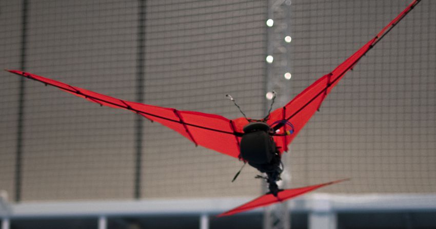
considering the formula of this coefficient, it can also be Fig. 2. Image of the reference prototype
simplified as ε = εα α, being εα = 0.3 in this case. Then, it
is obtained a lift coefficient given by
π III. R ESULTS AND DISCUSSION
CLt = [α (1 − εα ) + δt ] At (9) In order to see the evolution of the variables during
2
with δt being the deflection of the tail and At the aspect the transitional phase to the steady state, the ornithopter
ratio of the tail. However, these formulas are only valid in prototype showed in Fig. 2 has been used as reference.
the steady state. Whenever angular velocities appear, there The aerodynamic surfaces of this UAV are made of fabric
are unsteady effects which produce additional aerodynamics stiffened by carbon fiber ribs and spar, so aerodynamic theory
forces. They can be modelled at the typical Reynolds num- used is reasonable as the wing can be considered as a rigid
bers of the UAV by the linear potential theory of unsteady flat plate.
thin airfoils [25]. Neglecting the small terms associated to This vehicle has the capacity of alternating gliding and
the second temporal derivatives and to the weak effects of flapping modes but this paper is mainly focused on the
the unsteady wakes of wings and tail, they can be written as gliding mode, as one of the great advantages of birds consists
on their ability to travel long distances without flapping their
! wings. The values of the non-dimensional parameters for
1.5α̇ − 2lcw q A the prototype are written in Table I. All the results reported
CLus = 2π (10)
Ub A+2 below are obtained with these values.
!
π 1.5α̇ − 2lct q TABLE I
CLtus = At (11) M AGNITUDES OF THE UAV
2 Ub
where the dot denotes temporal derivative. The above coeffi- M Λ L RHL χ Li A At
cients are added to the ones in (8) and (9) in order to obtain 5.80 0.221 −9.60 1.12 0.133 0.005 4.78 2.35
the total forces. Unsteady aerodynamic does not affect the
steady state, as these are only transitional effects, but it is
fundamental in the evolution to that state, as they work as The results analysed are focused on showing the effects
damping terms in the glider dynamics. The pitch term comes of the unsteady aerodynamics on the gliding dynamics of
from the vertical displacement of the wing or tail produced the bio-inspired UAV. Firstly, the effect of these terms
by the rotation around the center of gravity with angular are analysed by comparing the evolution of the system of
velocity q, whereas the angle of attack rate term is produced equations with and without them. Then, a stability analysis
by the rotation of the velocity vector with respect to the wing is proposed by means of the linearisation of the model,
or tail. comparing the stability modes obtained.
As discussed in [19], stall of the lifting surfaces may
lead to unphysical results. For this reason, a procedure of A. Effect of unsteady aerodynamics
saturating the lift coefficients has been followed, reducing To better understand the effect that the unsteady aerodi-
also the effects of the unsteady terms when the saturation namic coefficients (10)-(11) have on the vehicle’s dynamics,
conditions are reached. As explained in [19], these limita- the equations (1)-(4) have been solved numerically with and
tions are established at relatives angles of attack of 15o for without these unsteady aerodynamic terms. The computation
the wing and 35o for the tail. has been done by using the ode45 function integrated in
Finally, induced drag is modelled from Prandtl’s lifting MATLAB (The MathWorks, Inc., Natick, MA, USA).
line theory in the linear limit as Table II shows the different sets of initial conditions used
2 2 in the numerical simulations, all of them with the same
CLs CLts
CDi = , CDit = (12) control variable (tail angle δt ), thus sharing the same gliding
πA πAt steady state (see [19]), which is also given in Table II. Note
where the subscript ”s” means the steady part of these that dimensional variables are used in this section, with the
coefficients, defined in (8) and (9). same name as their dimensionless counterparts. Initial point
1598
Authorized licensed use limited to: Universidad de Sevilla. Downloaded on January 20,2021 at 14:09:20 UTC from IEEE Xplore. Restrictions apply.Fig. 3. Comparison between trajectories considering and neglecting Fig. 4. Comparison between evolution of the trajectory angle considering
unsteady aerodynamic, being X the longitudinal distance and h the height and neglecting unsteady aerodynamic.
with respect to the Earth inertial frame.
of the trajectory is defined at 0 in the longitudinal frame
and a height of 75 m. Trajectories obtained with the first
two sets of initial conditions are compared in Fig. 3, and
results prove that oscillations in the trajectory of the system
considering only steady aerodynamics are growing, until
the computation is stopped as it reaches values where the
model lose its applicability. However, the model considering
unsteady coefficients reach the steady values.
TABLE II
D IMENSIONAL STATES
Initial conditions
Ub (m/s) γ(o ) q θ(o ) Fig. 5. Comparison between evolution of the velocity module considering
x10 4.08 0 0 0 and neglecting unsteady aerodynamic.
x20 12.23 −30 0 −20
x30 12.23 20 0 20
x40 4.08 0 0 10 figures is plotted in Fig. 8 in a phase diagram, where it is
x50 12.23 5 0 10 clearly shown that these two variables, which are the most
x60 8.15 0 0 −5 critical ones during the transient period, always converge
Steady state to the to the steady state. In some cases, short period can
Ub (m/s) γ(o ) q θ(o ) also be observed as the first displacement in this diagram
xs 6.00 −5.02 0 0.40 is not always following the spiral, for instance, with initial
conditions 2 and 6.
The divergence of the system without considering the B. Linearisation of the model
transient aerodynamic terms is clearer in the trajectory angle In order to numerically characterize the transition of the
shown in Fig. 4 for the same initial conditions. The am- gliding until reaching the steady state, a linearisation of
plitude of the oscillations of the model without unsteady the model is proposed, with the objective of obtaining the
aerodynamic terms becomes very high even at the first peak, stability modes. State variables are decomposed into a steady
and then blows up after a few oscillations, while when state and a perturbation:
the unsteady terms are taken into account low amplitude
oscillations converge towards the steady state. A similar
behaviour is observed for the speed (Fig. 5). Ub = Ubs + Ub (t) (13)
Figures 6 and 7 show the trajectory angle and the speed γ = γs + γ(t) (14)
obtained considering the unsteady terms with all the different q = qs + q(t) (15)
initial conditions given in Table II, thus showing that the
θ = θs + θ(t) (16)
ornithopter is capable of reaching the steady state for a wide
range of initial conditions. The information in these two δt = δts + δt (t) (17)
1599
Authorized licensed use limited to: Universidad de Sevilla. Downloaded on January 20,2021 at 14:09:20 UTC from IEEE Xplore. Restrictions apply.Fig. 9. Comparison between evolution of the trajectory angle given by the
non-linear model and the linear approximation.
Fig. 6. Comparison of the evolution of the trajectory angle for different
initial conditions.
After substituting this decomposition into (1)-(4), they
are linearised assuming small perturbations. Once the steady
state terms are eliminated, the following descriptor (implicit)
state-space model of linear equations is obtained for the
perturbations:
U̇b Ub
γ̇ γ
M = A + Bδt (18)
q̇ q
θ̇ θ
Note that we have selected the tail angle δt as the control
parameter. Matrices M , A and B are given by
CXU̇ 0 0 0
b
0 CZγ̇ 0 CZθ̇
M = (19)
0 Cmγ̇ Cmq̇ Cmθ̇
Fig. 7. Comparison of the evolution of the speed for different initial 0 0 0 1
conditions.
CXUb CXγ 0 CXθ
C CZγ CZq CZθ
A = ZUb (20)
0 Cmγ Cmq Cmθ
0 0 1 0
CXδt
CZδt
B= (21)
Cmδ
t
0
The coefficients depend of the equilibrium state chosen,
which is obtained by the deflection of the tail. The definitions
of each coefficient are formulated in Appendix I.
Figures 9 and Fig. 10 show the difference between the
non-linear and linear models for the trajectory angle and
speed, respectively. Results are quite similar, particularly
in the damping of the system and the frequency of the
Fig. 8. Phase diagram for speed and trajectory angle with different initial response. Overshooting of both variables gives the highest
conditions. error, which makes sense, because when the state is far from
the linearisation point the approximation is less accurate.
1600
Authorized licensed use limited to: Universidad de Sevilla. Downloaded on January 20,2021 at 14:09:20 UTC from IEEE Xplore. Restrictions apply.Fig. 11. Comparison between the eigenvalues λ = λr +iλi in the complex
plane obtained obtained with a without transient terms. The inset shows a
zoom around the imaginary axis.
Fig. 10. Comparison between evolution of the velocity module given by
the non-linear model and the linear approximation.
the simpler steady model has a pair of complex eigenvalues
with positive real part, which causes the divergence of the
The effect of each variable are related to diverse physical transient dynamics. In Fig. 11 right these small values are
effects. Velocity affects by means of the variation of the clearer, as a zoom has been made near the imaginary axis.
absolute aerodynamics forces. There is no velocity term in The eigenvalues obtained when considering the unsteady
the third equation as all the terms in (3) are aerodynamic aerodynamics are presented in Table III (to provide a more
forces. physical information, we give the dimensional values for the
The angle of attack is represented in the variations of γ ornithopter with characteristics summarized in Table I):
and θ, and it affects in two ways: variation of aerodynamic
coefficients and change of projections of the forces. In fact, TABLE III
the static stability coefficient Cmα is also in the equations E IGENVALUES OF THE SYSTEM
as it is the same as Cmθ . Coefficients of γ include also the
change of the gravity force projections. Unsteady aerodynamics considered
Unsteady aerodynamic is represented by the terms of q, γ̇ λ1 λ2 λ3,4
and θ̇. Those coefficients are responsible of the damping of −40.70 s−1 −10.76 s−1 −0.1943 ± 0.8162i s−1
the system. CXV̇ and CZγ̇ include the mass of the system, Unsteady aerodynamics neglected
whereas Cmq̇ corresponds to the moment of inertia. λ1,2 λ3,4
The control derivatives are related to the deflection of the −9.27 ± 4.61 s−1 0.224 ± 2.184 s−1
tail, being the only control variable of the UAV of Fig. 2
in gliding mode. However, in the present gliding analysis,
the effects of these terms is not going to be considered, as
TABLE IV
the focus here is on the free response of the glider, which is
E IGENVECTORS OF THE SYSTEM
obtained just with the variables of the system. For the cases
studied, the numerical values of the matrices are collected
in the Appendix II. They correspond to the dimensionless Unsteady aerodynamics considered
parameters in Table I and for the steady state defined in x01 x02 x03,04
Table II U b0 −0.0289 0.0853 0.9853∠0.9o
γ0 −0.1890 1 0.3404∠86.1o
C. Stability modes q0 1 0.0174 0.0103∠1.3o
The free-response of the solutions of the system (18) θ0 −0.5762 −0.0185 0.3433∠104.7o
(without the forcing term δt ), can be written as x = x0 eλt . Unsteady aerodynamics neglected
Considering this solution, the different modes are obtained x01,02 x03,04
solving the generalised eigenvalue problem given by U b0 0.1652∠140.5o 0.7629∠17.7o
γ0 1∠180.0o 0.6930∠120.4o
|M−1 A − λI| = 0. (22) q0 0.1962∠−1.5o 0.0573∠36.9o
θ0 0.5288∠152.1o 0.7286∠121.1o
−1
The eigenvalues and eigenvectors of the matrix M A
characterize the dynamic stability of the glider. The eigenval-
ues λ, obtained numerically in MATLAB using the function The eigenvectors associated to these modes are given in
eig, are plotted in the complex plane in Fig. 11. As Table IV. From these values it is possible to compare the
expected, the system with the unsteady aerodynamic coeffi- stability modes of the UAV as function of the unsteady
cients has all the eigenvalues with negative real part, whereas aerodynamic terms:
1601
Authorized licensed use limited to: Universidad de Sevilla. Downloaded on January 20,2021 at 14:09:20 UTC from IEEE Xplore. Restrictions apply.• Fast modes: In the case of neglecting the unsteady
aerodynamic, there is a single mode, an oscillatory
convergence, mainly associated to angular variables.
However, considering these terms, two exponential con-
vergences appear, related to the angular acceleration and
the trajectory angle. The dynamic is considerably fast
with both models, as times to reduce to half amplitude
with the updated model are of 0.0170 s and 0.0644 s,
similar to 0.0747 s associated to the other system.
These modes are related to the short period mode of
an airplane, but their effects are different in both cases.
When just the steady aerodynamic is considered, the
angular pitch velocity seems not to be damped, when
in aircraft is one of the most relevant of this mode. In the
other case, due to the differences in the design between Fig. 12. Evolution of the trajectory angle for the fast modes.
a regular fixed-wing aircraft and a bio-inspired vehicle,
the short period is overdamped. It is relevant that the
aerodynamic surfaces take almost all the plantform of
the ornithopter which causes this overdamping of the
mode.
In Fig. 12, evolution of the trajectory angle shows the
fast convergence of these modes. It also proves that the
convergence is exponential, with a faster and a slower
time.
• Slow modes: These are the modes which appear in
Figures 4-10. Neglecting the unsteady aerodynamics,
the mode is an oscillatory divergence, due to the lack
of damping terms for the reacting moments of the
glider. When these coefficients are considered, the mode
changes becoming stable. Some reference values of the
mode are written in Table V, where ωn is the natural
frequency, ξ the damping, t1/2 the time to damp to half Fig. 13. Evolution of the trajectory angle for the slow modes.
amplitude and t2 the time to duplicate the perturbations.
These characteristic values are clearly visible in Figures
4-10, particularly the frequencies and the times to damp IV. C ONCLUSIONS
or duplicate the perturbations. Due to the limitations of on-board instrumentation of
bio-inspired systems, complex aerodynamic models or full
TABLE V aerodynamic simulations are impossible to implement for
C HARACTERISTIC VALUES OF PHUGOID MODE real-time control. These vehicles require of simpler analytical
Unsteady aerodynamics considered models as it had been stated in [19]. This study intends
ωn ξ t1/2 to complement this previous work by the extension of the
0.84 rad/s 0.232 3.57 s validity of the model to unsteady cases.
Unsteady aerodynamics neglected
In this sense, the results presented here shows that the
ωn ξ t2
dynamics of the model of [19] diverge before reaching the
2.20 rad/s −0.102 3.10 s steady state, even when the system is statically stable. The
update presented here, which includes unsteady aerodynam-
ics coefficients, causes the system to converge to the steady
This mode is similar to the phugoid of a conventional state, taking values with much more physical meaning. It is
aircraft. From the eigenvectors associated, it is notice- worth mentioning that even if results for other prototypes
able that trajectory angle and pitch angle have a very may show convergence without the unsteady aerodynamics
similar module and a small difference of phase, meaning coefficients, neglecting them would affect trajectories ob-
that the variations on the angle of attack is significantly tained by simulations, showing a slower convergence.
smaller than these other angles. The linearisation of the model around the steady state
Fig. 13 shows the convergent oscillations of the trajec- allows to obtain a numerical characterization of the dynamic
tory angle in different phases. The characteristics seen stability of the system, in order to visualize the unsteady ef-
in Table V are clearly visible. The phugoid is the main fects more clearly. By this process, results show that phugoid
evolution seen in Figures 3-10. mode is unstable when unsteady aerodynamic effects are
1602
Authorized licensed use limited to: Universidad de Sevilla. Downloaded on January 20,2021 at 14:09:20 UTC from IEEE Xplore. Restrictions apply.
neglected, but it became stable when they are considered. 2 2πA πAt
CZγ = −Ubs +Λ (1 − εα )
Results also show that the short period is overdamped, A+2 2
which makes sense considering that the relative size of the + sin (γs ) (34)
aerodynamics surfaces respect to the total vehicle size is
2
more important than that of an aircraft. This characteristic Cmγ = Ubs (CLs + LΛCLts ) sin (αs )
also makes more relevant considering unsteady aerodynamics
2πA πAt
in bio-inspired UAVs. − + LΛ (1 − εα ) cos (αs )
A+2 2
The longitudinal model considered in this paper is quite
4CLs
more general, to our knowledge, than any other one consid- − + LΛCLts (1 − εα ) sin (αs )
ered before for modelling gliding ornithopters. Linearisation A+2
is also an important step towards an efficient control of − (CDs + ΛCDts ) cos (αs )
the gliding flight, allowing to reach and maintain a certain 2πA
+ RHL sin (αs ) + CLs cos (αs )
angle of trajectory and optimizing the distance traveled. A+2
In order to extend this work it would be appropriated to 4CLs
obtain experimental data and confirm that the stability modes − cos (αs ) + CDs sin (αs ) (35)
A+2
obtained theoretically corresponds to the actual flight. In
2 4CLs
this line, the work could also be extended to characterize CXθ = −Ubs + ΛCLts (1 − εα ) (36)
the stability of flapping phases in combined gliding and A+2
flapping flight. For that task it would be appropriated to use 2 2πA πAt
CZθ = Ubs +Λ (1 − εα ) (37)
a simplification for the flapping state, in order to characterize A+2 2
all the phases of the flight. 2
Cmθ = Ubs − (CLs + LΛCLts ) sin (αs )
A PPENDIX I 2πA πAt
+ + LΛ (1 − εα ) cos (αs )
L INEARISATION COEFFICIENTS A+2 2
4CLs
+ + LΛCLts (1 − εα ) sin (αs )
A+2
CXU̇ = 2M (23) + (CDs + ΛCDts ) cos (αs )
b
1 2πA
Cmq̇ = (24) − RHL sin (αs ) + CLs cos (αs )
χ A+2
A At
4CLs
CZγ̇ = Ubs 2M + 3π + Λ3π (25) − cos (αs ) + CDs sin (αs ) (38)
A+2 4 A+2
A At
Cmγ̇ = Ubs 3π + LΛ3π cos (αs )
A+2 4 2
CXδt = −ΛUbs CLts (39)
A
−RHL 3π sin (αs ) (26) 2 πA t
A+2 CZδt = ΛUbs (40)
A At
2
CZθ̇ = −Ubs 3π + Λ3π (27) 2 πAt
A+2 4 Cmδt = ΛUbs L cos (αs ) + CLts sin (αs ) (41)
2
A At
Cmθ̇ = −Ubs 3π + LΛ3π cos (αs )
A+2 4 A PPENDIX II
A
D ESCRIPTOR STATE - SPACE MODEL
−RHL 3π sin (αs ) (28)
A+2
The numerical values of the used in the simulations of
CXUb = −2Ubs (CDs + Li + ΛCDts ) (29) section III-C are the following
CZUb = 2Ubs (CLs + ΛCLts ) (30)
2πA 2lw lt
CZq = Ubs − − ΛπAt (31) 11.61 0 0 0
A+2 c c
0 28.62 0 −11.56
2πA 2lw lt M = (42)
Cmq = Ubs − − LΛπAt cos (αs )
A+2 c c
0 −8.46 30.07 8.46
2πA 2lw
0 0 0 1
+RHL sin (αs ) (32)
A+2 c −0.12 −0.40 0 −0.60
1.36 −10.89
4CLs 1.71 10.80
2 A= (43)
CXγ = Ubs + ΛCLts (1 − εα )
A+2
0 3.73 −39.58 −3.73
− cos (γs ) (33) 0 0 1 0
1603
Authorized licensed use limited to: Universidad de Sevilla. Downloaded on January 20,2021 at 14:09:20 UTC from IEEE Xplore. Restrictions apply.[22] A. Paranjape, N. K. Sinha and N. Ananthkrishnan, “Use of bifurcation
and continuation methods for aircraft trim and stability analysis - a
−0.09 state-of-the-art,” 45th AIAA Aerospace Sciences Meeting and Exhibit,
1.76
2007.
B= (44) [23] J. M. Dietl and E. Garcia, “Stability in ornithopter longitudinal flight
−16.90 dynamics,” Journal of Guidance, Control, and Dynamics, vol. 31, no.
0 4, pp. 1157–1163, 2008.
[24] D. McLean, Automatic flight control systems, Prentice Hall, 1990.
[25] J. Katz and A. Plotkin, Low-Speed Aerodynamics, Cambridge Univer-
R EFERENCES sity Press, 2001.
[26] A. L. Thomas, “On the aerodynamics of birds’ tails,” Philosophical
[1] C. J. Pennycuick, Modelling the flying bird, Elsevier, 2008. Transactions of the Royal Society of London. Series B: Biological
[2] U. M. Norberg, Vertebrate flight: mechanics, physiology, morphology, Sciences, vol. 340, no. 1294, pp. 361–380, 1993.
ecology and evolution. Springer, 2012. [27] R. T. Jones, Wing Theory, Princeton University Press, 1990.
[28] A. Silverstein and S. Katzoff, “Design charts for predicting downwash
[3] R. Dudley, The biomechanics of insect flight: form, function, evolution.
angles and wake characteristics behind plain and flapped wings,”
Princeton University Press, 2002.
NACA-Report No. 648, 1915.
[4] B. W. Tobalske, “Biomechanics of bird flight,” Journal of Experimen-
tal Biology, vol. 210, no. 18, pp. 3135–3146, 2007.
[5] U. L. Norberg, “Flight and scaling of flyers in nature,” Flow Phenom-
ena in Nature, vol. 1, pp. 120–154, 2007.
[6] C. P. Ellington, “The novel aerodynamics of insect flight: applications
to micro-air vehicles,” Journal of experimental biology, vol. 202, no.
23, pp. 3439–3448, 1999.
[7] J. A. Grauer and J. E. Hubbard, “Multibody model of an ornithopter,”
Journal of guidance, control, and dynamics, vol. 32, no. 5, pp.
1675–1679, 2009.
[8] H. E. Taha, M. R. Hajj, and A. H. Nayfeh, “Flight Dynamics and
Control of Flapping-Wing MAVs: A Review,” Nonlinear Dynamics,
vol. 70, pp. 907–939, 2012.
[9] Q.-V. Nguyen and W. L. Chan, “Development and flight performance
of a biologically-inspired tailless flapping-wing micro air vehicle with
wing stroke plane modulation,” Bioinspiration & biomimetics, vol. 14,
no. 1, p. 016015, 2018.
[10] A. Paranjape, S. J. Chung and M. S. Selig, “Flight mechanics of a
tailless articulated wing aircraft,” Bioinspiration & Biomimetics, vol.
6, no. 2, pp. 026005, 2011.
[11] C. Pennycuick, “Thermal soaring compared in three dissimilar tropical
bird species, fregata magnificens, pelecanus occidentals and cor-
agyps atratus,” Journal of Experimental Biology, vol. 102, no. 1, pp.
307–325, 1983.
[12] C. Pennycuick, “Soaring behaviour and performance of some east
african birds, observed from a motor-glider,” Ibis, vol. 114, no. 2,
pp. 178–218, 1972.
[13] P. Henningsson and A. Hedenström, “Aerodynamics of gliding flight
in common swifts,” Journal of experimental biology, vol. 214, no. 3,
pp. 382-393, 2011.
[14] P. Henningsson, A. Hedenström and R. J. Bomphrey, “Efficiency of
Lift Production in Flapping and Gliding Flight of Swifts,” PLOS ONE,
vol. 9, no. 2, pp. 1-7, 2014.
[15] A. Paranjape, M. R. Dorothy, S. J. Chung and K. D. Lee, “A flight
mechanics-centric review of bird-scale flapping flight,” International
journal of aeronautical and space science, vol. 13, no. 3, pp. 267-282,
2012.
[16] J. S. Lee, J. K. Kim, D. K. Kim and J. H Han, “Longitudinal
flight dynamics of bio-inspired ornithopter considering fluid-structure
integration,” Journal of guidance, control and dynamics, Vol. 34, no.
3, pp. 667-677, 2011.
[17] J. W. Roberts, R. Cory and R. Tedrake, “On the controllability of
fixed-wing perching,” 2009 American Control Conference, St. Louis,
MO, pp. 2018-2023, 2009.
[18] R. Cory and R. Tedrake, “Experiments in Fixed-Wing UAV Perching,”
AIAA Guidance, Navigation and Control Conference and Exhibit,
2008
[19] A. Martin-Alcantara, P. Grau, R. Fernandez-Feria and A. Ollero,
“A simple model for gliding and low-amplitude flapping flight of
a bio-inspired UAV,” 2019 International Conference on Unmanned
AircraftSystems (ICUAS), pp. 729-737, 2019.
[20] A. Thomas and G. Taylor, “Animal flight dynamics I. longitudinal
stability in gliding flight,” Journal of theoretical biology, vol. 212, no.
3, pp. 399–424, 2001.
[21] J. R. Usherwood, J. A. Cheney, J. Song, S. P. Windsor, J. P. J.
Stevenson, U. Dierksheide, A. Nila and R. J. Bomphrey, “High
aerodynamic lift from the tail reduces drag in gliding raptors,” Journal
of experimental biology, vol. 223, no. 3, 2020.
1604
Authorized licensed use limited to: Universidad de Sevilla. Downloaded on January 20,2021 at 14:09:20 UTC from IEEE Xplore. Restrictions apply.You can also read