Algebraic entropy fixes and convex limiting for continuous finite element discretizations of scalar hyperbolic conservation laws
←
→
Page content transcription
If your browser does not render page correctly, please read the page content below
Algebraic entropy fixes and convex limiting for continuous finite element
                                                           discretizations of scalar hyperbolic conservation laws

                                                                           Dmitri Kuzmina,∗, Manuel Quezada de Lunab
                                                                 a
                                                                     Institute of Applied Mathematics (LS III), TU Dortmund University
                                                                               Vogelpothsweg 87, D-44227 Dortmund, Germany
                                                                       b
                                                                         King Abdullah University of Science and Technology (KAUST)
arXiv:2003.12007v1 [math.NA] 26 Mar 2020

                                                                                      Thuwal 23955-6900, Saudi Arabia

                                           Abstract
                                           In this work, we modify a continuous Galerkin discretization of a scalar hyperbolic conservation law
                                           using new algebraic correction procedures. Discrete entropy conditions are used to determine the
                                           minimal amount of entropy stabilization and constrain antidiffusive corrections of a property-preserving
                                           low-order scheme. The addition of a second-order entropy dissipative component to the antidiffusive
                                           part of a nearly entropy conservative numerical flux is generally insufficient to prevent violations of
                                           local bounds in shock regions. Our monolithic convex limiting technique adjusts a given target flux in a
                                           manner which guarantees preservation of invariant domains, validity of local maximum principles, and
                                           entropy stability. The new methodology combines the advantages of modern entropy stable / entropy
                                           conservative schemes and their local extremum diminishing counterparts. The process of algebraic flux
                                           correction is based on inequality constraints which provably provide the desired properties. No free
                                           parameters are involved. The proposed algebraic fixes are readily applicable to unstructured meshes,
                                           finite element methods, general time discretizations, and steady-state residuals. Numerical studies of
                                           explicit entropy-constrained schemes are performed for linear and nonlinear test problems.
                                           Keywords: hyperbolic conservation laws, entropy stability, invariant domain preservation, finite
                                           elements, algebraic flux correction, convex limiting

                                           1. Introduction

                                               Entropy stability [8, 29, 33, 34] and preservation of invariant domains [14, 16, 19] play an important
                                           role in the design of numerical methods for nonlinear hyperbolic conservation laws. A failure to
                                           comply with these design criteria may result in nonphysical artefacts and/or convergence to wrong
                                           weak solutions. Modern high-resolution schemes are commonly equipped with flux or slope limiters

                                             ∗
                                              Corresponding author
                                              Email addresses: kuzmin@math.uni-dortmund.de (Dmitri Kuzmin), manuel.quezada@kaust.edu.sa (Manuel
                                           Quezada de Luna)

                                                                                                                                         March 27, 2020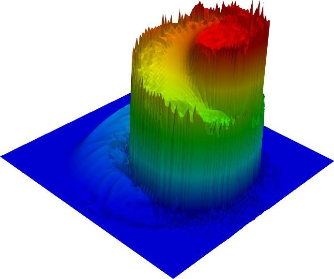
which guarantee the validity of discrete maximum principles but may fail to satisfy entropy conditions.
On the other hand, entropy stability of a high-order method does not guarantee the invariant domain
preservation (IDP) property and numerical solutions may exhibit undershoots/overshoots.
    Recent years have witnessed an increased interest of the finite element community in analysis and
design of algebraic flux correction (AFC) schemes [5, 6, 20, 21]. The AFC methodology modifies a
standard Galerkin discretization by adding artificial diffusion operators and limited antidiffusive fluxes.
The convex limiting techniques proposed in [14, 19, 22] are applicable to nonlinear hyperbolic problems
and lead to high-order IDP approximations. However, additional inequality constraints must be taken
into account to ensure entropy stability. In the context of finite volume and discontinuous Galerkin
(DG) approximations, entropy stability is commonly achieved by adding some entropy viscosity to
an entropy conservative numerical flux. For a comprehensive review of entropy stable schemes based
on this design philosophy, we refer to Tadmor [33, 34]. A representation of continuous finite element
approximations in terms of numerical fluxes is also possible [30, 31] but rather uncommon and requires
the use of edge-based data structures [25]. Therefore, the use of formulations that add diffusive fluxes
to the residual of the Galerkin discretization is preferred in the AFC literature [20].
    As shown by Guermond et al. [15], entropy stability is an essential requirement for convergence
of AFC schemes to correct weak solutions of nonlinear hyperbolic problems. Residual-based entropy
viscosity [14, 15] was found to be a good way to stabilize flux-corrected continuous Galerkin (CG)
approximations [14, 22]. However, it involves a free parameter and does not guarantee entropy stability.
The entropy fixes proposed by Abgrall et al. [1, 2] use Rusanov-type dissipation terms to enforce a cell
entropy inequality. In contrast to finite volume and DG methods, construction of entropy conservative
CG schemes for which this inequality holds as equality is an open problem. Hence, the minimal
amount of entropy stabilization needs to be determined without enforcing local entropy conservation.
The entropy stability conditions that we use in the present paper are derived by adapting Tadmor’s
[33] design criteria to the CG setting. The key ingredients of the proposed methodology are
   • inequality constraints that guarantee entropy stability and preservation of invariant domains;
   • a general framework for designing algebraic flux correction schemes based on such constraints;
   • new parameter-free algorithms for construction and limiting of entropy stabilization terms.
We begin with the CG space discretization of the initial value problem in Section 2. After introducing
the new AFC tools and their theoretical foundations in Sections 3-5, we summarize the proposed
algorithm in Section 6, perform numerical studies in Section 7, and draw conclusions in Section 8.

2. Finite element discretization
   Let u(x, t) be a scalar conserved quantity depending on the space location x ∈ Rd , d ∈ {1, 2, 3}
and time instant t ≥ 0. Consider an initial value problem of the form
                                   ∂u
                                      + ∇ · f (u) = 0      in Rd × R+ ,                               (1a)
                                   ∂t
                                        u(·, 0) = u0       in Rd ,                                    (1b)

                                                    2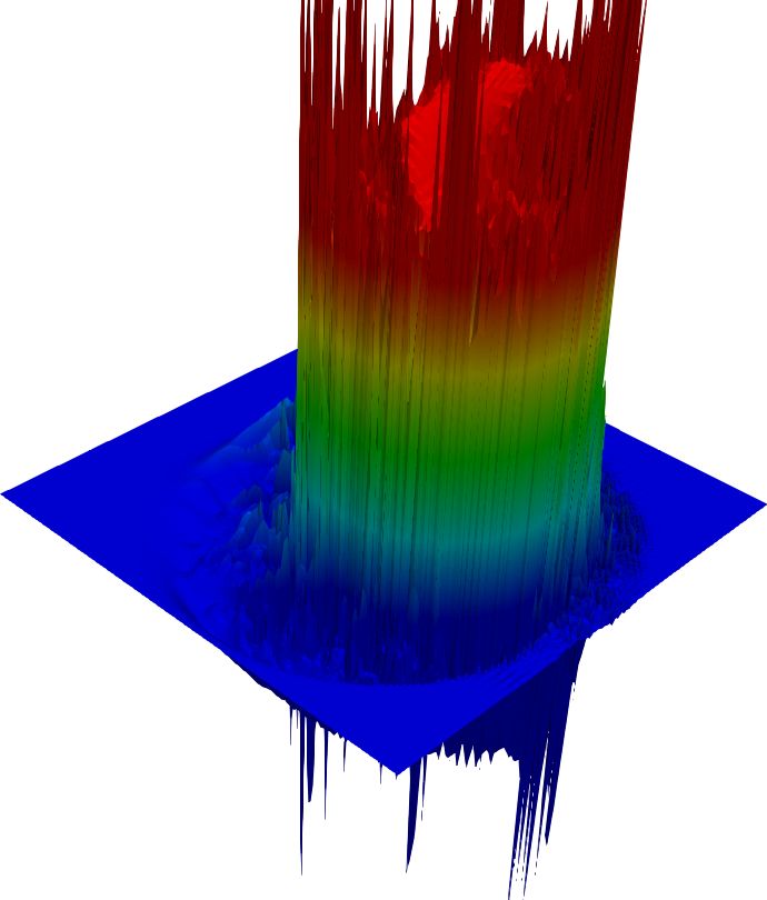
where f = (f1 , . . . , fd ) is a possibly nonlinear flux function and u0 : Rd → G is an initial data belonging
to a convex set G. The set G is called an invariant set of problem (1a)–(1b) if the exact solution u
stays in G for all t > 0 [16]. A convex function η : G → R is called an entropy and v = η 0 is called
an entropy variable if there exists an entropy flux q : G → Rd such that v(u)f 0 (u) = q0 (u). A weak
solution u of (1a) is called an entropy solution if the entropy inequality

                                               ∂η
                                                  + ∇ · q(u) ≤ 0             in Rd × R+                                  (2)
                                               ∂t
holds for any entropy pair (η, q). For any smooth weak solution, the conservation law

                                               ∂η
                                                  + ∇ · q(u) = 0             in Rd × R+                                  (3)
                                               ∂t
can be derived from (1a) using multiplication by the entropy variable v, the chain rule, and the definition
of an entropy pair. Hence, entropy is conserved in smooth regions and dissipated at shocks.
     Adopting the terminology of Guermond et al. [14, 16], we will call a numerical scheme invariant
domain preserving (IDP) if the solution of the (semi-)discrete problem is guaranteed to stay in an
invariant set G. Additionally, a property-preserving discretization of (1a) should be entropy stable,
i.e., it should satisfy a discrete version of the entropy inequality (2). The lack of entropy stability is a
typical reason for convergence of numerical schemes to nonphysical weak solutions.
     Restricting the spatial domain to Ω ⊂ Rd and imposing periodic boundary conditions for simplicity,
we discretize (1a) in space using a conforming mesh Th = {K1 , . . . , KEh } of linear (P1 ) or multilinear
(Q1 ) finite elements. The globally continuous basis functions ϕ1 , . . . , ϕNh are associated with the
vertices x1 , . . . , xNh of Th . Let Ei denote the set of (numbers of) elements containing the vertex xi
and N e is the setSof (numbers of) nodes belonging to K e . The computational stencil of node i is the
integer set Ni = e∈Ei N e . Substituting the finite element approximations

                                                   Nh
                                                   X                        Nh
                                                                            X
                                            uh =         uj ϕj ,     fh =         fj ϕj ≈ f (uh )                        (4)
                                                   j=1                      j=1

into the weak form of (1a) and using ϕi , i ∈ {1, . . . , Nh } as a test function, we obtain [19]
                      X X                   duj    X X                X                   X
                                     meij       =−      ceij · fj = −                               ceij · (fj − fi ),   (5)
                                             dt
                      e∈Ei   j∈N e                    e
                                                     e∈Ei j∈N                     e∈Ei j∈N e \{i}

                          Z                                    Z                        X
               meij   =           ϕi ϕj dx,         ceij   =        ϕi ∇ϕj dx,                 ϕj (x) = 1 ∀x ∈ K e .     (6)
                             Ke                                Ke                      j∈N e

The choice of the time integration method should ensure at least conditional L2 stability of the fully
discrete problem for linear flux functions of the form f (u) = vu, v ∈ Rd . The lack of nonlinear stability
can be cured using the algebraic flux correction tools that we present in the next sections.

                                                                      3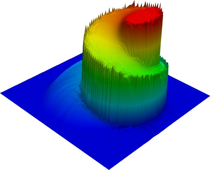
3. Property-preserving flux correction

   To enforce entropy inequalities and local discrete maximum principles, we approximate (5) by
                             X            dui   X            X
                                    mei       =                       e
                                                                    [gij − ceij · (fj − fi )],            (7)
                                          dt
                             e∈Ei                e∈Ei j∈N e \{i}

where                                                                   Z
                                                     X
                                           mei   =           meij   =        ϕi dx                        (8)
                                                     j∈N e              Ke

                                                                e are numerical fluxes such that
are the diagonal entries of the lumped element mass matrix and gij
                                     e      e
                                    gji = −gij           ∀i ∈ N e , j ∈ N e \{i}.                         (9)

The standard continuous Galerkin scheme (5) can be written in the form (7) using the fluxes
                                              e,CG
                                             gij   = meij (u̇i − u̇j ).                               (10)

The nodal time derivatives u̇i = du    i
                                     dt are defined by (5). To avoid inversion of the consistent mass
matrix, an approximate solution of this linear system for u̇ can be obtained efficiently using a few
Richardson’s iterations preconditioned by the lumped mass matrix [10, 26]. This approach to calcu-
lating u̇ corresponds to an approximation by a truncated Neumann series [15, 26].
                                                                   e,CG
    The purpose of algebraic flux correction (AFC) is to replace gij    with a flux that contains enough
numerical dissipation to ensure preservation of invariant domains, validity of local discrete maximum
principles and/or entropy stability. On the other hand, the levels of numerical diffusion should be
kept small enough to achieve optimal convergence behavior for problems with smooth exact solutions.
Similarly to PDE-constrained optimization problems, AFC schemes are designed to adjust the control
            e in a way which guarantees the validity of certain constraints for the state variables u
variables gij                                                                                          i
while staying as close as possible to a given target. Numerical solution of global constrained optimiza-
                                                                      e using sufficient conditions (box
tion problems is feasible [7] but costly. Therefore, we will design gij
constraints) to derive simple closed-form approximations which provide the desired properties.
   Let (η, q) be an entropy pair and v = η 0 (u) the corresponding entropy variable. Define

                                            ψ(u) = v(u)f (u) − q(u).                                  (11)

A sufficient condition for entropy stability of the semi-discrete problem (7) is given by (cf. [8, 27])
                           vi − vj e
                                  [gij − ceij · (fj + fi )] ≤ ceij · [ψ(uj ) − ψ(ui )].               (12)
                              2
In the following Theorem, we show that (12) implies the validity of a semi-discrete entropy inequality.

                                                               4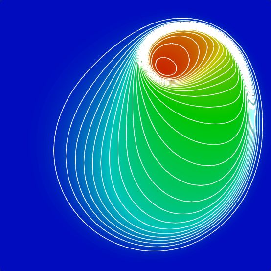
e , then
Theorem 1 (Entropy stability of AFC schemes [14, 16]). If condition (12) holds for each flux gij
the solution of the semi-discrete problem (7) satisfies the discrete entropy inequality
                                   X            dη(ui )   X         X
                                          mei           ≤                  [Geij − ceij · (qj − qi )],                     (13)
                                                  dt
                                   e∈Ei                    e∈Ei j∈N e \{i}

where
                                             vi + vj e      vi − vj e
                                           Geij =   gij −            cij · (fj − fi ).                                (14)
                                                2               2
Proof. We have e∈Ei mei dη(u         i)
                                        = e∈Ei mei vi du                                   e       e
                   P                       P                    P           P
                                                        dt =      e∈Ei vi     j∈N e \{i} [gij −cij ·(fj −fiP
                                                                                                           )] by the chain
                                                          i
                                  dt
                                                              0
rule and the definition of the entropy variable vi = η (ui ). Using the zero sum property j∈N e ceij = 0
of the discrete gradient operator, and the stability condition (12), we find that
             X                                      X
                     e
        vi         [gij − ceij · (fj − fi )] = vi            e
                                                          [gij  − ceij · (fj + fi )] − 2vi ceii · fi
           j∈N e \{i}                                     j∈N e \{i}

               X      vi + vj e       e                  vi − vj e
         =                   [gij − cij · (fj + fi )] +           [gij − cij · (fj + fi )] − 2vi ceii · fi
                                                                          e
                         2                                    2
           j∈N e \{i}
             X  vi + vj
         ≤                   [gij − cij · (fj + fi )] + cij · [ψ(uj ) − ψ(ui )] − 2vi ceii · fi
                               e      e                    e
                         2
           j∈N e \{i}
             X  vi + vj
                               e
         =                   [gij − ceij · (fj + fi )] + ceij · [ψ(uj ) + ψ(ui )] − 2ceii · [vi fi − ψ(ui )]
                         2
           j∈N e \{i}
             X  vi + vj
                                            vi − vj

                              e     e
  (∗)    =                   gij − cij ·             (fj − fi ) + qj + qi      − 2ceii · qi
                         2                     2
           j∈N e \{i}
             X  vi + vj
                                            vi − vj
                                                                                  X
                              e     e
         =                   gij − cij ·             (fj − fi ) + qj − qi      =            [Geij − ceij · (qj − qi )].
               e
                         2                     2                                       e
            j∈N \{i}                                                                          j∈N \{i}

Summing over e ∈ Ei , we conclude that the assertion of the Theorem is true.

   By definition of ceij , we have         e              e
                                   P              P
                                     e∈Ei cij = −   e∈Ei cji if i or j is an interior node. Under the
assumption  of periodic boundary conditions, this property holds for all nodes. In particular, we have
        e = 0. Using the identity marked by (*) in the proof of Theorem 2, we obtain the estimate
P
      c
  e∈Ei ii

         Nh X                      Nh X
                                      Nh
         X               dηi       X     vi + vj X
                     mei       ≤                                 e
                                                               (gij    e
                                                                    + gji )                                                (15)
                         dt                        2
          i=1 e∈Ei                 i=1    j=1           e∈Ei
                                                               | {z }
                                          j>i                      =0
                                   Nh X
                                      Nh                                     X
                                   X             vi − vj                                                   X
                               −                         (fj − fi ) + qj + qi ·      (ceij + ceji ) −2qi ·      ceii = 0
                                                    2
                                   i=1    j=1                                   e∈Ei                       e∈Ei
                                          j>i                                   |       {z       }         | {z }
                                                                                           =0                =0

                                                                       5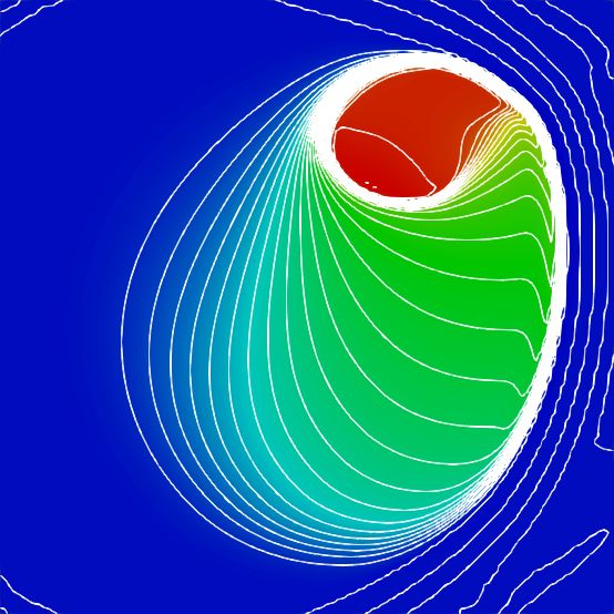
d
R
in accordance Rwith the fact that dt Ω η(u) dx ≤ 0 for the entropy solution of an initial boundary-value
problem with ∂Ω q(u) · n ds = 0, where n denotes the unit outward normal. Note that the validity of
2
estimate (15) for the square entropy η = u2 implies L2 stability.
Suppose that the exact entropy solution u belongs to a convex invariant set G = [umin , umax ]. Then
a semi-discrete scheme of the form (7) is invariant domain preserving (IDP) if it satisfies
umin ≤ umin max
i (t) ≤ ui (t) ≤ ui (t) ≤ umax ∀t ≥ 0. (16)
A fully discrete scheme possesses the IDP property if similar inequality constraints hold at each discrete
time level tn = n∆t, n ∈ N or stage of a strong stability preserving (SSP) Runge-Kutta method [12].
The following Theorem provides a sufficient condition for the design of IDP approximations.
Theorem 2 (Guermond-Popov IDP criterion [14, 16]). Consider a semi-discrete scheme of the form
X dui X X
mei = 2deij (ūeij − ui ), i ∈ {1, . . . , Nh }, (17)
dt
e∈Ei e∈Ei j∈N e \{i}
where mei > 0 and deij > 0 for all j ∈ N e \{i}. Let G be a convex set. Assume that
ui ∈ G, ūeij ∈ G ∀j ∈ N e \{i}. (18)
If the time step ∆t satisfies X X X
∆t 2deij ≤ mi = mei , (19)
e∈Ei j∈N e \{i} e∈Ei
then an explicit SSP Runge-Kutta time discretization of (17) is IDP w.r.t. G.
Proof. Each stage of an explicit SSP-RK method is a forward Euler update of the form
∆t X X
ūi = ui + 2deij (ūeij − ui )
mi
e∈Ei j∈N e \{i}
∆t X X ∆t X X
= 1 − 2deij ui + 2deij ūeij .
mi mi
e∈Ei j∈N e \{i} e∈Ei j∈N e \{i}
Under the time step restriction (19), this representation of the fully discrete scheme implies that ūi is
a convex combination of ui ∈ G and ūeij ∈ G. Since G is convex, the result ūi stays in G [16].
Remark 1. After the global residual assembly, the semi-discrete AFC scheme (7) becomes
dui X
mi = [gij − cij · (fj − fi )], (20)
dt
j∈Ni
6
where X X X
mi = mij , mij = meij , cij = ceij . (21)
j∈Ni e∈Ei ∩Ej e∈Ei ∩Ej
e e . However, the corrected
P
In this paper, we assemble gij = e∈Ei gij
from element contributions gij
flux can also be determined directly. In AFC schemes of this kind, inequality constraints for gij are
formulated using the coefficients of global matrices (cf. [14, 20, 19, 23]). All algorithms to be presented
below can be easily converted to the post-assembly format by dropping the superscript e.
4. Entropy stable AFC schemes
Let us begin with the derivation of semi-discrete AFC schemes satisfying the entropy stability
condition (12). A low-order approximation of local Lax-Friedrichs (LLF) type is defined by
e,LLF
gij = de,max
ij (uj − ui ), (22)
where
e |, |ce |} max{λmax , λmax } if i ∈ N e , j ∈ N e \{i},
max{|c
P ij ji ij ji
de,max
ij = − k∈N e \{i} deik if j = i ∈ N e , (23)
0 otherwise
are artificial diffusion coefficients proportional to the maximum wave speed [16, 19, 22]
ceij
λmax
ij = max |neij · f 0 (ωui + (1 − ω)uj )|, neij = . (24)
ω∈[0,1] |ceij |
The LLF flux defined by (22) satisfies (12), as shown by Chen and Shu [8] in the context of entropy
stable DG methods. Guermond and Popov [16] proved that the fully discrete SSP-RK version of
the LLF-AFC scheme is IDP and satisfies a discrete entropy inequality for any entropy pair (η, q).
However, the accuracy of the LLF approximation is first-order at best and significant amounts of
numerical diffusion can be removed without losing the entropy stability property.
e corresponding to a second-order entropy stable approximation, we adopt
To derive a flux control gij
Tadmor’s [32, 33] design philosophy which is based on comparison with entropy conservative schemes.
e,EC
Suppose that condition (12) holds as equality for some gij . Then it holds as inequality for
e,ES e,EC e
gij = gij + νij (vj − vi ), (25)
where νije ≥ 0 is an entropy viscosity coefficient. This simple comparison principle provides a powerful
tool for the design of entropy stable finite volume [11, 29, 34] and DG [8, 27] methods. For our AFC
e,EC e,EC
scheme (7) to be entropy conservative, the fluxes gij = −gji would need to satisfy
vi − vj e,EC
[gij − ceij · (fj + fi )] = ceij · [ψ(uj ) − ψ(ui )],
2
vi − vj e,EC
[gij + ceji · (fj + fi )] = ceji · [ψ(ui ) − ψ(uj )].
2
7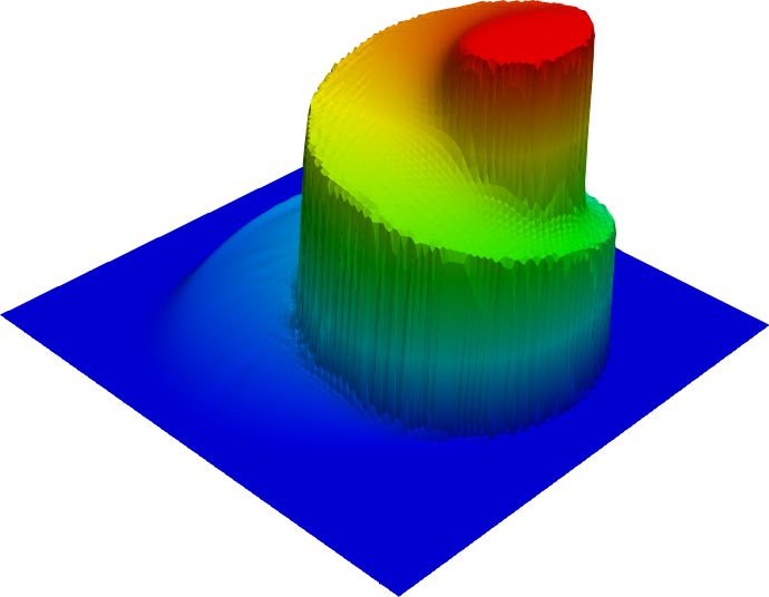
Since this system is overdetermined in the case ceij =6 −ceji , we perform element-level flux correction
using generalized entropy-stable target fluxes of the form
e,ES
gij = de,min
ij
e
(uj − ui ) + νij (vj − vi ), (26)
where de,min
ij ∈ [0, de,max
ij ] is the minimal nonnegative diffusion coefficient satisfying the symmetry
condition de,min
ij = de,min
ji and condition (12) for both nodes. The value of de,min
ij is given by
( min{Qe ,0,Qe }
ij ji
if ui 6= uj ,
de,min
ij = (vi −vj )(uj −ui ) (27)
0 if ui = uj ,
where
fj + fi
Qeij = 2ceij · ψ(uj ) − ψ(ui ) + (vi − vj ) . (28)
2
By the mean value theorem, we have vi − vj = η 0 (ui ) − η 0 (uj ) = η 00 (ξ)(ui − uj ) for some ξ ∈ R. It
follows that (vi − vj )(uj − ui ) ≤ 0 and, therefore, de,min
ij ≥ 0 for any convex entropy η.
Remark 2. In the absence of rounding errors, we have de,min
ij ≤ de,max
ij by definition. In practice,
division by a small number (vi − vj )(uj − ui ) may produce de,min
ij > de,max
ij in regions where the
numerical solution is almost constant. To avoid this, it is worthwhile to use de,max
ij as upper bound
for de,min
ij in practical implementations. We also remark that the direct calculation of the diffusive flux
min{Qeij ,0,Qeji }
de,min
ij (uj − ui ) = vi −vj is less sensitive to rounding errors in the limit |ui − uj | → 0.
The AFC scheme corresponding to (26) with νij e = 0 is barely entropy stable. Building on Tadmor’s
[33] ideas, we define the additional flux νije (v − v ) using the entropy viscosity coefficient
j i
h i h i
ceij · fj + fi − 2f uj +u
2
i
ce · f + f − 2f uj +ui
ji j i 2
e
νij = max , 0, (29)
vj − vi vi − vj
which vanishes for linear flux functions f (u) and preserves second-order accuracy for nonlinear ones.
Remark 3. For reasons explained in Remark 2, we recommend direct calculation of the flux
e
(vj − vi ) = Sij max Sij ceij · 2∆fij , 0, −Sij ceji · 2∆fij ,
νij (30)
u +u
where Sij is the sign of vj − vi and ∆fij = 12 (fj + fi ) − f j 2 i is the flux difference.
The use of (26) with de,min
ij
e defined by (29) yields an entropy stable approxi-
defined by (27) and νij
mation which exhibits the desired convergence behavior for smooth data but may produce undershoots
and/or overshoots in the neighborhood of shocks. To enforce the IDP property and preservation of
local bounds, we use the monolithic convex limiting techniques presented in the next section.
8
5. Bound-preserving AFC schemes
The highly dissipative LLF flux (22) satisfies not only the entropy condition (12) but also the
assumptions of Theorem 2. The corresponding IDP bar states are given by
uj + ui ceij · (fj − fi )
ūeij = − , (31)
2 2de,max
ij
where de,max
ij is defined by (23). Using the mean value theorem, one can show that [19]
min{ui , uj } ≤ ūeij ≤ max{ui , uj }. (32)
Hence, the algebraic LLF scheme is IDP by Theorem 2. To limit the raw antidiffusive part
e,LLF
fije = gij
e
− gij (33)
e in a manner which preserves the IDP property, we define
of a given flux control gij
e,∗ e,LLF
gij = gij + fije,∗ = de,max
ij (uj − ui ) + fije,∗ (34)
using the inequality-constrained antidiffusive flux [19, 22]
n o
min fije , 2deij min {umax
i − ūeij , ūeji − umin
j } if fije > 0,
e,∗
fij = n o (35)
max fije , 2deij max{umin
i − ūeij , ūeji − umax
j } otherwise.
This monolithic convex limiting (MCL) strategy was proposed in [19]. It guarantees that
fij∗
min uj =: umin ≤ ūe,∗ e
ij = ūij + ≤ umax := max uj . (36)
j∈Ni
i
2de,max
ij
i
j∈Ni
The IDP property of the flux-corrected scheme can be shown using Theorem 2, see [19] for details.
Remark 4. A linearity-preserving version of the bounds umin i and umax
i can be constructed as proposed
in Section 6.1 of [19]. The use of limiters that guarantee linearity preservation (i.e., produce fije,∗ = fije
for locally linear functions uh ) is essential for achieving optimal convergence to smooth solutions [4].
Formula (35) will leave the raw antidiffusive flux fije unchanged if it does not violate the AFC
inequality constraints (36). Hence, the quality of flux-corrected solutions depends on the properties of
the (stabilized) high-order method defined by (7) with gije = g e,LLF + f e . The target flux
ij ij
fije = (de,min
ij − de,max
ij
e
)(uj − ui ) + νij (vj − vi ) (37)
9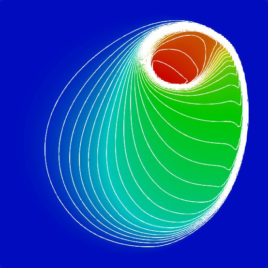
e,LLF
corresponds to an entropy stable lumped-mass approximation. The addition of (37) to gij replaces
e,ES
it with gij . If limiting is performed using (35), the addition of fije,∗ replaces gij
e,LLF
with
e,∗
fij if fije 6= 0,
e,∗ e e,max e,ES e e
gij = (1 − αij )dij (uj − ui ) + αij gij , αij = fij (38)
0 otherwise.
Recall that (vi − vj )(uj − ui ) ≤ 0 for any convex entropy η by the mean value theorem and definition
e ∈ [0, 1] and de,max ≥ de,min , we have
of the entropy variable v = η 0 (u). Since αij ij ij
e,∗
(vi − vj )gij e
= (vi − vj )[(1 − αij )de,max
ij
e e,min
(uj − ui ) + αij e e
dij (uj − ui ) + αij νij (vj − vi )]
≤ (vi − vj )de,min
ij (uj − ui ).
e,LLF e,∗
Thus the replacement of gij by gij produces an entropy stable and bound-preserving approximation.
In the consistent-mass version of our AFC scheme, the target flux to be used in (35) is given by
fije = meij (u̇i − u̇j ) + (de,min
ij − de,max
ij
e
)(uj − ui ) + νij (vj − vi ) (39)
e = g e,CG + g e,ES . The nodal time derivatives u̇ can be defined
and represents the antidiffusive part of gij ij ij
using (5) or (7). In the numerical examples of Section 7, we use the LLF approximation
1 X X
u̇i = [de,max
ij (uj − ui ) − ceij · (fj − fi )]. (40)
mi e
e∈Ei j∈N \{i}
In addition to being rather inexpensive, it has the positive effect of introducing high-order background
stabilization [19] even for linear advection problems, for which νij e defined by (29) vanishes.
The inclusion of mij (u̇i − u̇j ) may require additional limiting of fije,∗ to ensure that the final flux
e
e,∗∗ e,LLF
gij = gij + fije,∗∗ = de,max
ij (uj − ui ) + fije,∗∗ (41)
of our property-preserving AFC scheme (7) will satisfy the entropy stability condition
vi − vj e,∗∗
[gij − ceij · (fj + fi )] ≤ ceij · [ψ(uj ) − ψ(ui )]. (42)
2
Substituting (41) into (42), we obtain a limiting criterion for the algebraic entropy fix
( min{Qe,∗ ,(v −v )f e,∗ ,Qe,∗ }
if (vi − vj )fije,∗ > 0,
ij i j ij ji
e,∗∗ vi −vj
fij = (43)
fij∗ otherwise,
where
Qe,∗ e e,max
ij = Qij − (vj − vi )dij (ui − uj ) (44)
are upper bounds for entropy-producing fluxes. The value of Qeij is given by (28). Note that
Qe,∗ e,max
ij ≥ (vi − vj )(dij
e,min
− dij )(ui − uj ) = η 00 (ξ)(de,max
ij − de,min
ij )(ui − uj )2
for some ξ ∈ R. Since de,max
ij ≥ de,min
ij , the bounds Qe,∗
ij are nonnegative for any convex entropy η.
10Remark 5. The replacement of fije,∗ by the entropy-corrected flux fije,∗∗ is equivalent to multiplication
e ∈ [0, 1]. Hence, it does not affect the IDP property of our AFC scheme.
by a correction factor αij
6. Summary of the algorithm
Let us now summarize the algorithmic steps to be performed and the properties of the AFC scheme
that ensures entropy stability and preservation of local bounds. At the semi-discrete level, the flux-
corrected CG approximation is defined by the nonlinear system of ordinary differential equations
dui
[de,max (uj − ui ) + fije,∗∗ − ceij · (fj − fi )],
X X
mi = ij i = 1, . . . , Nh , (45)
dt e
e∈Ei j∈N \{i}
where de,max
ij is the maximal speed diffusion coefficient defined by (23). If all corrections are included,
the computation of the limited antidiffusive flux fije,∗∗ involves the following steps:
1. Calculate the minimal diffusion coefficient de,min
ij using (27).
2. Calculate the e
entropy viscosity coefficient νij using (29).
3. Calculate the approximate time derivatives u̇i using (40).
4. Calculate the raw antidiffusive fluxes fije using (39).
5. Calculate the local bounds umax
i and umin
i using (36).
6. Calculate the bound-preserving fluxes fije,∗ using (35).
7. Calculate the entropy-corrected fluxes fije,∗∗ using (43).
The following implication of Theorem 2 provides a sufficient condition for an explicit time discretization
of the nonlinear semi-discrete AFC problem (45) to be locally bound preserving.
Theorem 3 (IDP property of the flux-corrected CG scheme). An explicit SSP Runge-Kutta time
discretization of system (45) satisfies the local maximum principle
umin
i ≤ ūi ≤ umax
i (46)
under the time step restriction
2de,max
X X
∆t ij ≤ mi . (47)
e∈Ei j∈N e \{i}
Proof. To apply Theorem 2, we notice that each SSP Runge-Kutta stage can be written as (cf. [19])
∆t X
2de,max (ūe,∗∗
X
ūi = ui + ij ij − ui ), (48)
mi
e∈Ei j∈N e \{i}
where
fije,∗∗
umin ≤ ūe,∗∗ = ūeij + ≤ umax (49)
i ij
2de,max
ij
i
by virtue of (32), (35), and (43). The desired result follows by the convexity argument.
11Remark 6. The applicability of the presented AFC tools is not restricted to explicit SSP Runge-Kutta
time discretizations. Nonlinear discrete problems associated with implicit time discretizations and the
steady state limit of (45) can be analyzed as in [5, 24], see also the Appendix of [19].
7. Numerical examples
In this section, we perform numerical experiments for linear and nonlinear scalar problems. The
purpose of this numerical study is to demonstrate that the proposed methodology provides optimal
accuracy for linear (P1 ) and multilinear (Q1 ) finite element approximations to smooth solutions, and
that it behaves as expected on structured as well as unstructured meshes. In the description of the
numerical results, we use the abbreviation LO-ES-IDP for the low-order LLF scheme defined by (7)
and (22). The high-order entropy stable IDP scheme of Section 6 is labeled HO-ES-IDP. The method
corresponding to HO-ES-IDP without Step 6 is referred to as HO-ES. We use this version to show
the effect of deactivating the IDP limiter. The significance of individual steps of the HO-ES-IDP
algorithm is further illustrated by varying the definition of the target flux fije for a two-dimensional test
problem with a nonconvex flux function (the so-called KPP problem [18]). In all numerical examples,
we discretize in time using the third-order explicit SSP Runge-Kutta method with three stages [12].
Unless otherwise stated, we use structured triangular meshes. All computations are performed using
Proteus (https://proteustoolkit.org), an open-source Python toolkit for numerical simulations.
7.1. One-dimensional advection
The first problem that we consider in this work is the one-dimensional linear advection equation
∂u ∂u
+a = 0 in Ω = (0, 1) (50)
∂t ∂x
with the constant velocity a = 1. The smooth initial condition is given by
u0 (x) = cos (2π(x − 0.5)) . (51)
We solve (50) up to the final time t = 1 and measure the numerical errors w.r.t. the L1 norm. In
Table 1, we show the results of a grid convergence study. As expected, LO-ES-IDP exhibits first-order
convergence behavior, while second-order convergence is achieved with HO-ES and HO-ES-IDP.
7.2. Two-dimensional advection
The next example was used in [3] to study the numerical behavior of flux-corrected transport
algorithms for high-order DG discretizations of the two-dimensional linear advection problem
∂u
+ v · ∇u = 0 in Ω = (0, 100)2 (52)
∂t
with constant velocity v = (10, 10). The initial condition, which is shown in Figure 1b, is composed of
two rings and a cross. The upper ring is centered at (x, y) = (40, 40). The radii of its inner and outer
12LO-ES-IDP HO-ES HO-ES-IDP
Nh kuh − uexact kL1 EOC kuh − uexact kL1 EOC kuh − uexact kL1 EOC
11 3.70E-2 – 1.21E-2 – 1.69E-2 –
16 2.92E-2 0.58 6.01E-3 1.73 8.32E-3 1.74
21 2.40E-2 0.68 3.73E-3 1.65 5.15E-3 1.66
31 1.77E-2 0.75 1.82E-3 1.76 2.51E-3 1.77
41 1.40E-2 0.81 1.08E-3 1.81 1.47E-3 1.84
61 9.84E-3 0.86 5.06E-4 1.86 6.93E-4 1.86
81 7.59E-3 0.90 2.95E-4 1.88 4.01E-4 1.90
121 5.21E-3 0.92 1.36E-4 1.89 1.87E-4 1.88
161 3.97E-3 0.94 7.86E-5 1.91 1.08E-4 1.90
241 2.68E-3 0.96 3.65E-5 1.89 4.94E-5 1.92
321 2.03E-3 0.97 2.11E-5 1.90 2.82E-5 1.94
481 1.36E-3 0.98 9.69E-6 1.91 1.28E-5 1.95
Table 1: One-dimensional advection. Grid convergence history for three entropy-stable AFC schemes.
circles are 7 and 10, respectively. The center of the lower ring is located at the point (x, y) = (40, 20).
The radii of the inner and outer circles are 3 and 7, respectively. The cross occupies the region
r1 ∪r2 ⊂ Ω, where r1 = {x, y ∈ Ω | x ∈ [7, 32], y ∈ [10, 13]} and r2 = {x, y ∈ Ω | x ∈ [14, 17], y ∈ [3, 26]},
rotated by −45◦ around the point (x, y) = (15.5, 11.5).
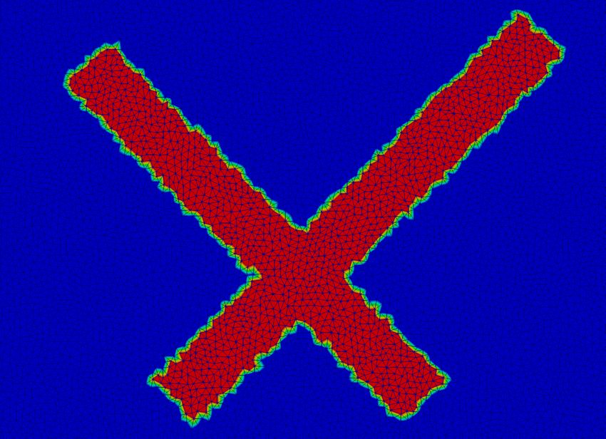
For this problem, we use unstructured grids. In Figure 1a, we show a zoom of one of these grids.
Computations are terminated at the final time t = 4. In Figures 1c and 1d, we present the LO-
ES-IDP and HO-ES solutions calculated using Nh = 99, 412 degrees of freedom (DoFs). The higher
accuracy of the latter approximation illustrates the need for antidiffusive corrections of the LLF flux.
No significant undershoots or overshoots are generated by HO-ES in this example. The results obtained
with the HO-ES-IDP scheme on three successively refined meshes are shown in Figure 2. The advected
discontinuities are resolved in a crisp and nonoscillatory manner, especially on the finest mesh.
umax = 0.5034 umax = 0.9862
(a) zoom of the grid (b) initial condition (c) LO-ES-IDP solution (d) HO-ES solution
Figure 1: Two-dimensional linear advection problem. Zoom of the unstructured grid, initial data, and numerical solutions
at t = 4 obtained with Nh = 99, 412 DoFs.
13umax = 0.9382 umax = 0.9947 umax = 0.9999
(a) Nh = 99, 412 (b) Nh = 395, 745 (c) Nh = 1, 580, 651
Figure 2: Two-dimensional linear advection problem. Numerical solutions at t = 4 obtained with HO-ES-IDP on three
successively refined unstructured grids.
7.3. KPP problem
The KPP problem [16, 17, 18] is a challenging nonlinear test for verification of entropy stability
properties. We use this problem to test different components of the method that we propose. In this
series of 2D experiments, we solve equation (1a) with the nonlinear and nonconvex flux function
f (u) = (sin(u), cos(u)) (53)
in the computational domain Ω = (−2, 2) × (−2.5, 1.5) using the initial condition
( p
14π
4 if x2 + y 2 ≤ 1,
u0 (x, y) = π (54)
4 otherwise.
A simple (but rather pessimistic) upper bound for the guaranteed maximum speed (GMS) is λ = 1.
More accurate GMS estimates can be found in [17]. The exact solution exhibits a two-dimensional
rotating wave structure, which is difficult to capture in numerical simulations using high-order methods.
The main challenge of this test is to prevent possible convergence to wrong weak solutions.
Numerical solutions are evolved up to the final time t = 1. To test individual components of the
AFC scheme summarized in Section 6, we vary the definition of the target flux fije and/or the way in
which it is limited to produce a constrained flux fije,∗∗ . In Figure 3a, we present the LO-ES-IDP solution
(fije,∗∗ = 0 = fije ). It is highly dissipative but provides a correct qualitative description of the rotating
wave structure. The solution displayed in Figure 3b was calculated using fije,∗∗ = deij (ui −uj ) = fije . This
lumped-mass Galerkin approximation is highly oscillatory and exhibits an entropy-violating merger of
two shocks. The solutions shown in Figures 3c and 3d were obtained using the IDP-limited counterparts
fije,∗∗ = fije,∗ of fije = deij (ui − uj ) and fije = meij (u̇i − u̇j ) + deij (ui − uj ), respectively. As reported in
[19, 24], the latter definition of the target flux introduces high-order background dissipation. However,
neither the activation of the IDP limiter nor the inclusion of meij (u̇i − u̇j ) provides enough entropy
dissipation to capture the twisted shocks correctly in the KPP test. This unsatisfactory state of affairs
14illustrates the need for entropy stabilization and confirms the findings of Guermond et al. [16] who
noticed that IDP limiting alone does not guarantee convergence to entropy solutions.
(a) (b) (c) (d)
Figure 3: Numerical solutions of the KPP problem at t = 1 obtained using Nh = 1292 DoFs and (a) LO-ES-IDP, (b)
e,∗∗
unconstrained lumped-mass Galerkin method corresponding to fij = de,max
ij
e
(ui − uj ) = fij , (c) IDP limiter (35) for
e,max
e
fij = dij (ui − uj ), and (d) IDP limiter (35) for fij = mij (u̇i − u̇j ) + de,max
e e
ij (u i − u j ).
In Figure 4, we present numerical solutions produced by three entropy stable high-order methods
using Nh = 1292 . Each column corresponds to a different definition of the target flux fije . The diagrams
of the first row were calculated without invoking the IDP flux limiter (35). Therefore, the results exhibit
undershoots/overshoots. The target fluxes of the three schemes under investigation are listed in the
caption. The use of fije = (de,min ij − de,max
ij )(uj − ui ) produces a barely entropy stable approximation
which requires additional entropy fixes to keep the shocks separated if no IDP constraints are imposed.
The inclusion of νije (v n − v n ) and me (u̇ − u̇ ) leads to AFC schemes that reproduce the rotating wave
j i ij i j
structure correctly even without IDP limiting. The method employed in the last diagram of the second
row is HO-ES-IDP. In Figure 5, we show the HO-ES-IDP results for finer meshes. As the number of
degrees of freedom is increased, the method converges to a bound-preserving entropy solution.
7.4. Inviscid Burgers equation
Let us now consider the two-dimensional inviscid Burgers equation [13, 19]
2
∂u u
+∇· v =0 in Ω = (0, 1)2 , (55)
∂t 2
where v = (1, 1) is a constant vector. The piecewise-constant initial data is given by
−0.2 if x < 0.5 ∧ y > 0.5,
−1.0 if x > 0.5 ∧ y > 0.5,
u0 (x, y) = (56)
0.5 if x < 0.5 ∧ y < 0.5,
0.8 if x > 0.5 ∧ y < 0.5.
15(a) (b) (c)
Figure 4: Numerical solutions of the KPP problem obtained at t = 1 using Nh = 1292 DoFs. The diagrams of the first
and second rows show the results produced by three entropy stable high-order schemes without and with activation of
the IDP flux limiter, respectively. The target fluxes are defined by (a) fij e
= (de,min
ij − de,max
ij )(un n
j − ui ) for the diagrams
e e,min e,max
of the first column, (b) fij = (dij − dij )(un n e n n
j − ui ) + νij (vj − vi ) for the diagrams of the second column, and (c)
e e e,min e,max e
fij = mij (u̇i − u̇j ) + (dij + dij )(uj − ui ) + νij (vj − vi ) for the diagrams of the third column.
(a) Nh = 2572 (b) Nh = 5132 (c) Nh = 10252
Figure 5: Numerical solutions of the KPP problem at t = 1 obtained using HO-ES-IDP on three meshes.
16The inflow boundary conditions are defined using the exact solution of the pure initial value problem
in R2 . This solution can be found in [13] and stays in the invariant set G = [−1.0, 0.8].
The final time for computation of numerical solutions is t = 0.5. In Table 2, we show the results
of a grid convergence study for LO-ES-IDP, HO-ES, and HO-ES-IDP. In this example, the low-order
LLF scheme performs remarkably well at self-steepening shocks but the resolution of rarefactions is
not as accurate as in the case of the high-order entropy stable method without and with IDP limiting.
The HO-ES-IDP results calculated on three successively refined meshes are displayed in Figure 6.
LO-ES-IDP HO-ES HO-ES-IDP
Nh kuh − uexact kL1 EOC kuh − uexact kL1 EOC kuh − uexact kL1 EOC
332 7.63E-2 – 4.02E-2 – 3.93E-2 –
652 4.49E-2 0.76 2.12E-2 0.92 2.09E-2 0.91
1292 2.51E-2 0.85 1.11E-2 0.95 1.10E-2 0.95
2572 1.37E-2 0.85 5.57E-3 0.97 5.62E-3 0.94
5132 7.31E-3 0.90 2.80E-3 0.99 2.83E-3 0.98
Table 2: Inviscid Burgers equation in two dimensions. Grid convergence history for three entropy stable AFC schemes.
(a) Nh = 332 (b) Nh = 1292 (c) Nh = 5132
Figure 6: Inviscid Burgers equation in two dimensions. Numerical solutions at t = 0.5 obtained with HO-ES-IDP on
three meshes. In each diagram, we plot 30 contour lines corresponding to a uniform subdivision of G = [−1.0, 0.8].
7.5. Buckley-Leverett equation
In the last numerical experiment, we consider the two-dimensional Buckley-Leverett equation. The
nonconvex flux function of the nonlinear conservation law to be solved is [9]
u2
1
f (u) = 2 . (57)
u + (1 − u)2 1 − 5(1 − u)2
17The computational domain is Ω = (−1.5, 1.5)2 . The initial condition is given by
(
1 if x2 + y 2 < 0.5,
u0 (x, y) = (58)
0 otherwise.
An upper bound for the fastest wave speed can be found in [9]. Similarly to the KPP problem, the
solution exhibits a rotating wave structure. In Figure 7, we show the entropy stable AFC approxima-
tions at the final time t = 0.5. Note that small oscillations are present if the IDP flux limiter is not
applied. The effect of mesh refinement on the accuracy of HO-ES-IDP is illustrated by the snapshots
presented in Figure 8. In all experiments for this test problem we use bilinear finite elements.
umax = 0.9469 umax = 1.0002 umax = 0.9923
(a) LO-ES-IDP (b) HO-ES (c) HO-ES-IDP
Figure 7: Two-dimensional Buckley-Leverett problem. Numerical solutions at t = 0.5 obtained with three entropy-stable
AFC schemes using Q1 finite elements and Nh = 1292 DoFs. In each diagram, we plot 30 contour lines corresponding to
a uniform subdivision of G = [0, 1].
8. Conclusions
We have shown that algebraic flux correction schemes can be configured to satisfy discrete entropy
inequalities in addition to discrete maximum principles. The new inequality-constrained stabilization
techniques modify the residual of the semi-discrete Galerkin scheme in a way which ensures entropy
stability while preserving all other important properties (conservation, preservation of local bounds, low
levels of numerical diffusion). The proposed methodology was presented in the context of continuous
Galerkin methods. Further developments will focus on the DG version [1, 2, 8, 27], extensions to
high-order finite elements [3, 22], and design of entropy stability preserving time integrators [28].
Acknowledgments. The work of Dmitri Kuzmin was supported by the German Research Association
(DFG) under grant KU 1530/23-1. The authors would like to thank Hennes Hajduk (TU Dortmund
University) for careful proofreading of the manuscript and helpful feedback.
18umax = 1 umax = 1 umax = 1
Figure 8: Two-dimensional Buckley-Leverett problem. Numerical solutions at t = 0.5 obtained with HO-ES-IDP on
three meshes. In each diagram, we plot 30 contour lines corresponding to a uniform subdivision of G = [0, 1].
References
[1] R. Abgrall, A general framework to construct schemes satisfying additional conservation relations.
Application to entropy conservative and entropy dissipative schemes. J. Comput. Phys. 372 (2018)
640–666.
[2] R. Abgrall, P. Öffner, and H. Ranocha, Reinterpretation and extension of entropy correction terms
for residual distribution and discontinuous Galerkin schemes. Preprint arXiv: 1908.04556v1,
2019
[3] R. Anderson, V. Dobrev, Tz. Kolev, D. Kuzmin, M. Quezada de Luna, R. Rieben, and V. To-
mov, High-order local maximum principle preserving (MPP) discontinuous Galerkin finite element
method for the transport equation. J. Comput. Phys. 334 (2017) 102–124.
[4] G. Barrenechea, V. John, and P. Knobloch, A linearity preserving algebraic flux correction scheme
satisfying the discrete maximum principle on general meshes. Mathematical Models and Methods
in Applied Sciences (M3AS) 27 (2017) 525–548.
[5] G. Barrenechea, V. John, and P. Knobloch, Analysis of algebraic flux correction schemes. SIAM
J. Numer. Anal. 54 (2016) 2427–2451.
[6] G. Barrenechea, V. John, P. Knobloch, and R. Rankin, A unified analysis of algebraic flux correc-
tion schemes for convection-diffusion equations. SeMA 75 (2018) 655–685.
[7] P. Bochev, D. Ridzal, M. D’Elia, M. Perego, and K. Peterson, Optimization-based, property-
preserving finite element methods for scalar advection equations and their connection to Algebraic
Flux Correction. Preprint, 2019, https://doi.org/10.13140/RG.2.2.20942.72000.
19[8] T. Chen and C.W. Shu, Entropy stable high order discontinuous Galerkin methods with suitable
quadrature rules for hyperbolic conservation laws. J. Comput. Phys. 345 (2017) 427–461.
[9] I. Christov and B. Popov, New non-oscillatory central schemes on unstructured triangulations for
hyperbolic systems of conservation laws. J. Comput. Phys. 227-11, (2008) 5736–5757.
[10] J. Donea, S. Giuliani, H. Laval, and L. Quartapelle, Time-accurate solution of advection-diffusion
equations by finite elements. Comput. Methods Appl. Mech. Engrg. 193 (1984) 123–145.
[11] U. Fjordholm, S. Mishra, and E. Tadmor, Energy Preserving and Energy Stable Schemes for
the Shallow Water Equations. In F. Cucker, A. Pinkus, and M. Todd (Eds.), Foundations of
Computational Mathematics, Hong Kong 2008 (London Mathematical Society Lecture Note Series,
pp. 93-139). Cambridge: Cambridge University Press, 2009.
[12] S. Gottlieb, C.-W. Shu, and E. Tadmor, Strong stability-preserving high-order time discretization
methods. SIAM Review 43 (2001) 89–112.
[13] J.-L. Guermond and M. Nazarov, A maximum-principle preserving C 0 finite element method for
scalar conservation equations. Computer Methods Appl. Mech. Engrg. 272 (2014) 198–213.
[14] J.-L. Guermond, M. Nazarov, B. Popov, and I. Tomas, Second-order invariant domain preserving
approximation of the Euler equations using convex limiting. SIAM J. Sci. Computing 40 (2018)
A3211-A3239.
[15] J.-L. Guermond, M. Nazarov, B. Popov, and Y. Yang, A second-order maximum principle pre-
serving Lagrange finite element technique for nonlinear scalar conservation equations. SIAM J.
Numer. Anal. 52 (2014) 2163–2182.
[16] J.-L. Guermond and B. Popov, Invariant domains and first-order continuous finite element ap-
proximation for hyperbolic systems. SIAM J. Numer. Anal. 54 (2016) 2466–2489.
[17] J.-L. Guermond and B. Popov, Invariant domains and second-order continuous finite element
approximation for scalar conservation equations. SIAM J. Numer. Anal. 55 (2017) 3120–3146.
[18] A. Kurganov, G. Petrova, and B. Popov, Adaptive semidiscrete central-upwind schemes for non-
convex hyperbolic conservation laws. SIAM J. Sci. Comput. 29 (2007) 2381–2401.
[19] D. Kuzmin, Monolithic convex limiting for continuous finite element discretizations of hyperbolic
conservation laws. Comput. Methods Appl. Mech. Engrg. 361 (2020) 112804.
[20] D. Kuzmin, Algebraic flux correction I. Scalar conservation laws. In: D. Kuzmin, R. Löhner and
S. Turek (eds.) Flux-Corrected Transport: Principles, Algorithms, and Applications. Springer, 2nd
edition: 145–192 (2012).
20[21] D. Kuzmin, M. Möller, and M. Gurris, Algebraic flux correction II. Compressible flow problems.
In: D. Kuzmin, R. Löhner, S. Turek (eds), Flux-Corrected Transport: Principles, Algorithms, and
Applications. Springer, 2nd edition, 2012, pp. 193–238.
[22] D. Kuzmin and M. Quezada de Luna, Subcell flux limiting for high-order Bernstein finite element
discretizations of hyperbolic conservation laws. J. Comput. Phys. Available online 21 March 2020,
109411, https://doi.org/10.1016/j.jcp.2020.109411
[23] D. Kuzmin and S. Turek, Flux correction tools for finite elements. J. Comput. Phys. 175 (2002)
525–558.
[24] C. Lohmann, Physics-Compatible Finite Element Methods for Scalar and Tensorial Advection
Problems. Springer Spektrum, 2019.
[25] R. Löhner, Applied CFD Techniques: An Introduction Based on Finite Element Methods (2nd
edition). John Wiley & Sons, Chichester, 2008.
[26] L. Quartapelle, Numerical Solution of the Incompressible Navier-Stokes Equations. ISNM 113,
Birkäuser, Basel, 1993.
[27] W. Pazner and P.-O. Persson, Analysis and entropy stability of the line-based discontinuous
Galerkin method. J. Scientific Computing 80 (2019) 376–402.
[28] H. Ranocha, M. Sayyari, L. Dalcin, M. Parsani, and D.I. Ketcheson, Relaxation Runge-Kutta
methods: Fully-discrete explicit entropy-stable schemes for the compressible Euler and Navier-
Stokes equations. Preprint arXiv:1905.09129 [math.NA], 2019.
[29] D. Ray, P. Chandrashekar, U.S. Fjordholm, and S. Mishra, Entropy stable scheme on two-
dimensional unstructured grids for Euler equations. Commun. Comput. Phys. 19 (2016) 1111–
1140.
[30] V. Selmin, The node-centred finite volume approach: bridge between finite differences and finite
elements. Comput. Methods Appl. Mech. Engrg. 102 (1993) 107–138.
[31] V. Selmin and L. Formaggia, Unified construction of finite element and finite volume discretizations
for compressible flows. Int. J. Numer. Methods Engrg. 39 (1996) 1–32.
[32] E. Tadmor, The numerical viscosity of entropy stable schemes for systems of conservation laws I.
Math. Comp. 49 (1987) 91–103.
[33] E. Tadmor, Entropy stability theory for difference approximations of nonlinear conservation laws
and related time-dependent problems. Acta Numerica (2003) 451–512.
[34] E. Tadmor, Entropy stable schemes. Handbook of Numerical Analysis, Vol. 17, Elsevier, 2016.
21You can also read