The Observational Uncertainty of Coronal Hole Boundaries in Automated Detection Schemes - IOPscience
←
→
Page content transcription
If your browser does not render page correctly, please read the page content below
The Astrophysical Journal, 913:28 (9pp), 2021 May 20                                                                https://doi.org/10.3847/1538-4357/abf2c8
© 2021. The Author(s). Published by the American Astronomical Society.

   The Observational Uncertainty of Coronal Hole Boundaries in Automated Detection
                                       Schemes
      Martin A. Reiss1 , Karin Muglach2,3 , Christian Möstl1 , Charles N. Arge2, Rachel Bailey4 , Véronique Delouille5,
      Tadhg M. Garton6, Amr Hamada7, Stefan Hofmeister8,9, Egor Illarionov10,11, Robert Jarolim8, Michael S. F. Kirk2,12 ,
         Alexander Kosovichev13,14,15 , Larisza Krista16,17 , Sangwoo Lee18, Chris Lowder19, Peter J. MacNeice2, and
                                                     Astrid Veronig8,20
                                   COSPAR ISWAT Coronal Hole Boundary Working Team
                                        1
                                          Space
                                              Research Institute, Austrian Academy of Sciences, Graz, Austria; martin.reiss@oeaw.ac.at
                                       2
                                      Heliophysics Science Division, NASA Goddard Space Flight Center, Greenbelt, MD 20771, USA
                                                      3
                                                        Catholic University of America, Washington, DC 20064, USA
                                         4
                                            Conrad Observatory, Zentralanstalt für Meteorologie und Geodynamik, Vienna, Austria
                                                             5
                                                               Royal Observatory of Belgium, Brussels, Belgium
                                                               6
                                                                 University of Southampton, Southampton, UK
                                7
                                  Space Physics and Astronomy Research Unit, Space Climate Group, University of Oulu, Oulu, Finland
                                                           8
                                                             University of Graz, Institute of Physics, Graz, Austria
                                          9
                                            Columbia Astrophysics Laboratory, Columbia University, New York, NY 10027, USA
                                                            10
                                                               Moscow State University, Moscow, 119991, Russia
                                           11
                                              Moscow Center of Fundamental and Applied Mathematics, Moscow, 119234, Russia
                                                                  12
                                                                     ASTRA llc, Louisville, CO 80027, USA
                                13
                                   Center for Computational Heliophysics, New Jersey Institute of Technology, Newark, NJ 07102, USA
                                          14
                                             Department of Physics, New Jersey Institute of Technology, Newark, NJ 07102, USA
                                                     15
                                                        NASA Ames Research Center, Moffett Field, CA 94035, USA
                           16
                              Cooperative Institute for Research in Environmental Sciences, University of Colorado, Boulder, CO 80309, USA
                    17
                       National Centers for Environmental Information, National Oceanic and Atmospheric Administration, Boulder, CO 80305, USA
                                                         18
                                                             Korean Space Weather Center, Jeju, Republic of Korea
                                                             19
                                                                Southwest Research Institute, Boulder, CO, USA
                                   20
                                      Kanzelhöhe Observatory for Solar and Environmental Research, University of Graz, Graz, Austria
                                               Received 2021 January 20; accepted 2021 March 25; published 2021 May 21

                                                                               Abstract
             Coronal holes are the observational manifestation of the solar magnetic field open to the heliosphere and are of
             pivotal importance for our understanding of the origin and acceleration of the solar wind. Observations from space
             missions such as the Solar Dynamics Observatory now allow us to study coronal holes in unprecedented detail.
             Instrumental effects and other factors, however, pose a challenge to automatically detect coronal holes in solar
             imagery. The science community addresses these challenges with different detection schemes. Until now, little
             attention has been paid to assessing the disagreement between these schemes. In this COSPAR ISWAT initiative,
             we present a comparison of nine automated detection schemes widely applied in solar and space science. We study,
             specifically, a prevailing coronal hole observed by the Atmospheric Imaging Assembly instrument on 2018 May
             30. Our results indicate that the choice of detection scheme has a significant effect on the location of the coronal
             hole boundary. Physical properties in coronal holes such as the area, mean intensity, and mean magnetic field
             strength vary by a factor of up to 4.5 between the maximum and minimum values. We conclude that our findings
             are relevant for coronal hole research from the past decade, and are therefore of interest to the solar and space
             research community.
             Unified Astronomy Thesaurus concepts: Solar physics (1476); Solar coronal holes (1484); Solar magnetic flux
             emergence (2000); Solar wind (1534); Solar extreme ultraviolet emission (1493); Solar magnetic fields (1503);
             Space weather (2037)

                                    1. Introduction                                      types include highly Alfvénic slow wind emerging from
                                                                                         coronal hole boundaries, and fast wind streams emerging from
   Coronal holes are an observational manifestation of open
                                                                                         slowly diverging field lines deep inside low-latitude coronal
magnetic field lines emerging from the solar photosphere into
                                                                                         holes and polar coronal hole extensions (Zirker 1977; Wang &
interplanetary space. The evolving ambient solar wind is
formed as coronal plasma escapes along these open field lines                             Sheeley 1990). At Earth, these fast solar wind streams can
into space. Depending on the location and strength of the                                interact with the magnetosphere, causing geomagnetic
heating along the open field lines, several types of solar wind                           disturbances (Krieger et al. 1973; Tsurutani et al. 2006).
originate from coronal holes (McComas et al. 2007). These                                   A defining feature of coronal holes is their reduced coronal
                                                                                         emission. Because the open field guides coronal plasma into
                                                                                         space, coronal holes are cooler and less dense than closed-field
                 Original content from this work may be used under the terms
                 of the Creative Commons Attribution 4.0 licence. Any further            regions. They therefore emit less radiation than the adjacent
distribution of this work must maintain attribution to the author(s) and the title       coronal plasma. Ground- and space-based instruments observe
of the work, journal citation and DOI.                                                   these reduced intensity regions at different wavelengths. The

                                                                                     1
The Astrophysical Journal, 913:28 (9pp), 2021 May 20                                                                                               Reiss et al.

Figure 1. Example coronal hole from 2018 May 30 observed by the Solar Dynamics Observatory. (a) Full-disk image of the Sun in the Fe XII (19.3 nm; T ≈ 1.6 MK)
emission line; (b)–(d) coronal hole under scrutiny in the Fe IX (17.1 nm; T ≈ 0.6 MK), Fe XII (19.3 nm; T ≈ 1.6 MK), and Fe XIV (21.1 nm; T ≈ 2.0 MK)
emission lines.

spectrum includes radio, near-infrared (particularly He I                         detection (Caplan et al. 2016). As a consequence, coronal
1083 nm), white light, EUV, and X-rays (see Newkirk 1967;                         hole boundaries computed from automated schemes, which
Munro & Withbroe 1972). Due to these collective observations                      deal with these hindrances differently, are expected to show
and advancements in instrumentation and remote sensing,                           inherent discrepancies.
coronal hole research has flourished over the past decades. This                      So a natural question arises: how large are the observational
research has covered plasma and magnetic properties (Zirker                       uncertainties of coronal hole boundaries in automated detection
1977; Cranmer 2009), temporal and spatial evolution, and the                      schemes? In 2019 the Coronal Hole Boundary Working
role played by coronal holes in modeling and predicting the                       Team21 in the COSPAR ISWAT initiative22 was formed to
ambient solar wind at Earth (Wang & Sheeley 1990; Riley et al.                    address this question. In this paper we present our first results.
2001; Arge et al. 2003).                                                          We compare nine established detection schemes applied to an
   Automated coronal hole detection schemes are of broad                          example coronal hole on 2018 May 30. We will show that the
interest to the community. Historically, He I images have been                    choice of scheme has a significant effect not only on the
used by observers to detect coronal holes by eye (Harvey &                        location of the coronal hole boundary but also on the inferred
Recely 2002; McIntosh 2003). The first automated coronal hole                      physical conditions inside the hole.
detection scheme using ground-based observations was devel-                          Our paper is outlined as follows. In Section 2, we present the
oped by Henney & Harvey (2005). Later, automated schemes                          example coronal hole on 2018 May 30. Section 3 describes the
using a combination of ground and space-borne observations                        solar imagery and automated detection schemes, while
were proposed (see, for instance, Malanushenko & Jones 2005;                      Section 4 presents the observational uncertainty of coronal
Toma & Arge 2005; Scholl & Habbal 2008). With approxi-                            holes in automated schemes. The discussion in Section 5
mately 70,000 images a day captured by the Solar Dynamics                         concludes this paper and outlines future perspectives.
Observatory (SDO; Pesnell et al. 2012) mission, the automated
detection of coronal holes is an important diagnostic in solar
and space science. Many unsolved questions in solar wind                                            2. A Case Study for 2018 May 30
physics, such as the mechanism for solar wind acceleration and
the origin of the slow solar wind, are intimately connected with                     To quantify the uncertainty of coronal hole boundaries in
coronal hole research (Kilpua et al. 2016; Viall & Borovsky                       automated detection schemes, we study an example low-
2020).                                                                            latitude coronal hole on 2018 May 30. As shown in Figure 1(a),
   But detecting coronal holes without human interaction is                       the hole is located near the disk center, southward of the active
challenging (Toma & Arge 2005). First, reduced coronal                            region AR 12712. Persistent for several solar rotations, it was
emission does not uniquely define coronal holes because                            first observed around 2017 November 24. Initially, the hole was
filaments and regions of weak magnetic flux appear at a similar                     connected to a southern polar coronal hole with negative
intensity; Reiss et al. (2015) showed that about 15% of coronal                   polarity as expected for solar cycle 24 (Lowder et al. 2017).
holes detected with automated schemes are not coronal holes.                      After the example shown for 2018 May 30, the coronal hole
Second, extracting coronal holes from photospheric magnetic                       was observable for five Carrington rotations before it
field measurements is impossible (Harvey & Sheeley 1979),                          disappeared.
coronal holes are expected to be predominantly of one polarity                       As shown in the Appendix, the coronal hole was associated
but not all holes show this textbook behavior (Hofmeister et al.                  with a high-speed stream in measurements by the Solar
2017, 2019). Third, the coronal hole appearance may vary                          Wind Electron Proton Alpha Monitor (SWEPAM; McComas
greatly between different EUV and SXR filters sensitive to                         et al. 1998) on board the Advanced Composition Explorer
different plasma temperatures, which makes a definition of                         (ACE; Stone et al. 1998) spacecraft. Starting at around
their boundaries difficult. Fourth, other important factors such                   2018 May 31 14:00 UT, the measurements show a gradual
as the noisy nature of EUV images, changes in viewing                             increase in bulk speed. On 2018 June 1 the solar wind speed
angle due to solar rotation (Wang 2017), overshining of                           peaked at around 700 km s−1. An increase in the magnetic field
coronal hole regions due to large nearby coronal loops
(Wang 2017), systematic instrument effects, and the spatial                       21
                                                                                       https://iswat-cospar.org/S2-01
                                                                                  22
and temporal evolution of coronal holes complicate their                               https://iswat-cospar.org

                                                                              2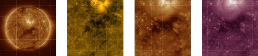
The Astrophysical Journal, 913:28 (9pp), 2021 May 20                                                                                           Reiss et al.

                                                                         Table 1
                                        Automated Coronal Hole Detection Schemes Widely Applied in the Community

Short            Research                         Reference                   Input                                               Online
Name             Institution                                                  Wave Band                                          Platform
(1)              (2)                              (3)                         (4)                                                   (5)
ASSA-CH          Korean Space Weather Center      Hong et al. (2012)          19.3 nm                               https://spaceweather.rra.go.kr/assa
CHARM            Trinity College                  Krista &                    19.3 nm, LOS magnetogram               https://github.com/lariszakrista/
                   Dublin; NOAA                     Gallagher (2009)                                                              CHARM
CHIMERA          Trinity College Dublin           Garton et al. (2018)        17.1 nm, 19.3 nm, 21.1 nm               https://github.com/TCDSolar/
                                                                                                                                CHIMERA
CHORTLE          Southwest Research Institute     Lowder et al. (2014)        19.3 nm, LOS magnetogram               https://github.com/lowderchris/
                                                                                                                                CHORTLE
CNN193           Moscow State University          Illarionov &                19.3 nm                               https://github.com/observethesun/
                                                     Tlatov (2018)                                                             coronal_holes
CHRONNOS         University of Graz               Jarolim et al. (2021)       9.4 nm, 13.1 nm, 17.1 nm,                              L
                                                                              19.3 nm, 21.1 nm, 30.4 nm, 33.5 nm,
                                                                              LOS magnetogram
SPoCA-CH         Royal Observatory of             Delouille et al. (2018)     19.3 nm                               http://swhv.oma.be/user_manual/
                   Belgium
SYNCH            University of Oulu               Hamada et al. (2018)        17.1 nm, 19.3 nm, 30.4 nm                             L
TH35                                              L                           19.3 nm                                               L

Note. TH35 is a baseline reference scheme against which future studies can be easily compared against.

and density lead to a minor geomagnetic disturbance with a                        groups to detect the coronal hole boundaries with each scheme.
maximum Kp of 5 and a minimum Dst of −38 nT.                                      By using the same data set for all the detection schemes, we
                                                                                  rule out discrepancies due to the preprocessing of the imagery.
                                                                                  The exception was the ASSA algorithm, which requires
                               3. Methods                                         preprocessed synoptic AIA images scaled down to 1024 ×
                3.1. Observational Data Preparation                               1024 pixels in JPG format.
   We use full-disk images in multiple EUV wave bands and
                                                                                                   3.2. Automated Detection Schemes
photospheric magnetic field measurements from the Atmo-
spheric Imaging Assembly (AIA; Lemen et al. 2012) and the                            We compare nine automated detection schemes widely
Helioseismic and Magnetic Imager (HMI; Scherrer et al. 2012)                      applied in coronal hole research. Table 1 lists these schemes
instruments on board the SDO spacecraft (Pesnell et al. 2012).                    along with their short name, institution, reference, input wave
Due to the high contrast between coronal holes and the adjacent                   bands, and online platform.
plasma, the AIA 19.3 nm wave band is most widely used. This                          Although each scheme aims to classify each pixel in a solar
filter is centered around the Fe XII emission line at 19.3 nm and                  coronal image as a coronal hole or background, the methods to
is dominated by the emission of plasma at around 1.6 MK. As                       do so are diverse. A common strategy is an intensity-based
illustrated in Figures 1(b)–(d), some automated schemes also                      thresholding due to the high contrast of coronal holes compared
use lower-temperature filters such as Fe IX 17.1 nm and                            to the rest of the coronal plasma, especially in the 19.3 nm
Fe XIV 21.1 nm.                                                                   wave band. The key is to find an intensity threshold that best
   We downloaded all images from the SDO data archive as                          separates the intensity distribution associated with coronal
level 1.0 data, to which basic data calibration methods had                       holes in a histogram. ASSA, for example, computes the
already been applied. Next, we used the SolarSoft 23 procedure                    intensity threshold equal to 45% of the median intensity on the
aia_prep.pro to apply geometric corrections like centering                        disk (Hong et al. 2012). In contrast, SPoCA-CH relies on an
the images, thereby removing shifts between the different AIA                     iterative clustering algorithm called fuzzy C-means, which
filters, correcting the roll angle to align E–W and N–S to the x-                  minimizes the variance in each cluster (Verbeeck et al. 2014).
and y-axis of the image, as well as scaling all images to                         The parameter setting used in the present study first determines
0.6 arcsec per pixel.                                                             the mode of the pixel intensity distribution, and then clusters in
   We use HMI measurements of the line-of-sight (LOS)                             four classes the intensities smaller than this mode. The class
component of the photospheric magnetic field. The LOS                              with lowest intensity determines the coronal hole locations
magnetogram (collected every 45 s) closest in time to the AIA                     (Delouille et al. 2018). These settings give different results
image was selected for analysis. We processed the HMI                             from what is currently implemented in the SDO Event
magnetogram with aia_prep.pro to apply the same                                   Detection System and the JHelioviewer.
geometric correction procedures. The HMI magnetogram,                                An alternative strategy uses thresholding by partitioning a
therefore, matches AIA down to less than a pixel. In this                         full-disk image into subframes. This reduces the overlap
way, we map the coronal hole boundaries onto the magneto-                         between different features in an intensity histogram and the
gram to retrieve photospheric magnetic field information.                          local minima are more clearly discernible. CHARM (Krista &
   We distributed the level 1.5 processed images as FITS files                     Gallagher 2009) and CHORTLE (Lowder et al. 2014) rely on
in the original size of 4096 × 4096 pixels to the participating                   this idea, searching for local minima in subframes of varying
                                                                                  sizes. Measures such as the mean of the local minima define
23
     https://sohowww.nascom.nasa.gov/solarsoft/                                   the global threshold. Furthermore, the intensity thresholding

                                                                              3
The Astrophysical Journal, 913:28 (9pp), 2021 May 20 Reiss et al.
method in CHARM also relies on the overall intensity of the field strength that is related to the heating of the corona and the
Sun, and hence the CH threshold detection adapts to the acceleration of the solar wind.
changing overall coronal emission over the solar activity cycle. Based on these two measures, the degree of unipolarity (U)
The SYNCH scheme searches for the subframe that is calculated using
separates coronal holes most clearly. This search is done in avg (∣BLOS∣) - ∣avg (BLOS)∣
three passbands (17.1, 19.3, 30.4 nm) in synoptic EUV maps, U= , (1 )
or alternatively in LOS disk images. The logical conjunction of avg (∣BLOS∣)
these three detections gives the final coronal hole map (Hamada where U = 0 represents a pure unipolar field and U = 1
et al. 2018). Since coronal holes are often present in all three represents a pure bipolar magnetic field (see Ko et al. 2014). It
passbands, such an approach should avoid incorrectly segmen-
can be understood intuitively as a measure of how much the
ted regions such as filaments. CHIMERA also uses three
passbands but does not partition the solar image into coronal hole differs from the expected textbook behavior.
subframes. Instead, the multithermal images are used to Furthermore, we study the open magnetic flux defined as
segment coronal holes by comparing the intensities across the N
three passbands. By computing a differentiation rule in the F= å BLOS
(i ) (i )
A , (2 )
intensity space, CHIMERA creates coronal hole maps in all i
three wave bands, and the logical conjunction gives the final where N is the total number of coronal hole pixels, BLOS (i )
is
map (Garton et al. 2018). magnetic field strength at each pixel, and A ( i)
is the
An original approach is taken in the CNN193 scheme. corresponding pixel area. In this context, Φ represents the net
CNN193 uses a neural network to detect coronal holes in the flux through the coronal hole regions detected by the schemes
19.3 nm wave band. The network is trained on a data set of
in units of Maxwell (Mx).
solar images and semiautomatically created segmentation
maps. Semiautomated means that the segmentation was done
4. Results
by an automated scheme but the results were supervised by an
experienced observer. In this way, the neural network is a In Figure 2, we present the coronal hole boundaries for the
surrogate for coronal hole detections done by an observer nine detection schemes on 2018 May 30, an example that is
(Illarionov & Tlatov 2018). challenging for automated schemes. An initial visual assess-
CHRONNOS also applies a neural network but uses all six ment shows that the different schemes produce significantly
EUV filtergrams of AIA and the HMI LOS magnetogram different outcomes. These differences are minimal around the
simultaneously as input to the network. As a reference, it builds dark regions denoting the center of the coronal hole, and most
upon manually reviewed SPoCA-CH segmentation masks from prominent farthest from the center. Smaller differences also
Delouille et al. (2018). With this approach, the identification of arise inside the coronal hole boundaries, most likely due to
the coronal holes and their boundaries is based on the ephemeral regions inside the coronal hole (see, for instance,
multichannel EUV appearance and the underlying magnetic Wang 2020).
field. The network uses a progressively growing approach to While all methods are capable of detecting the coronal hole,
include more spatial information, while also accounting for its size and form vary considerably. And these differences are
global relations in the full-disk observations (Jarolim et al. not only restricted to its shape; the physical properties of the
2021). coronal hole also show large differences.
To set a baseline against which future studies can easily be In Figure 3(a), we quantify the uncertainties in the observed
compared, we define a reference benchmark scheme called CH boundaries by assigning each pixel a number between
TH35. The intensity threshold is computed as 35% of the 0 and 9, which reflects how many times the pixel was
medium intensity on the solar disk, with no further postproces- identified belonging to the coronal hole: e.g., pixels with
sing of the coronal hole maps. 9 have been identified by all nine detection schemes to belong
For an in-depth review of the automated schemes, we refer to to the coronal hole. In Figure 3 we also show the contours
the references in Table 1. of the nine different CH boundaries over the AIA 19.3 nm
image (b) and the HMI magnetogram (c). All schemes capture
the darkest regions inside the boundary, but several also
3.3. Physical Properties in Coronal Holes
identify larger regions leading for instance to higher mean
We study the physical properties inside the detected coronal EUV emission.
holes using measures described in Ko et al. (2014). For the In Figure 4, we show the coronal hole properties derived
EUV data we focus on the mean intensity in the AIA 19.3 nm for the all detection schemes. Figure 4(a) shows the coronal
wave band (I193), which is the average intensity of all pixels hole area, which ranges from 33.59 × 10³ Mm2 to 151.24 ×
inside the CH boundary given in data numbers (DNs) per 103 Mm2. This means that the areas derived by the different
second. schemes vary by a factor of 4.5 between the minimum and
In addition, we study several measures computed from HMI maximum values. The mean AIA intensity in the 19.3 nm wave
magnetograms, such as the signed (BLOS) and unsigned (|BLOS|) band (b) varies between 14.84 DN s−1 and 31.18 DN s−1, with
magnetic field strength in Gauss (G) averaged over the area a factor of 2.1 between the maximum and minimum value.
outlined by the coronal hole boundary determined by each Similarly, the signed average field strength (c) ranges from
scheme. BLOS gives the net unbalanced field strength, which −1.21 G to −2.53 G, with a factor of 2.1 between the
cancels the background noise that we assume is present in equal maximum and minimum value. The unsigned average magnetic
measure in both polarities. As such, it is a robust measure of the field strength (d) ranges between values of 7.85 G and 8.50 G,
average field strength of the open field (Abramenko et al. 2009). with a factor of 1.1. The degree of unipolarity (e) ranges
On the other hand, |BLOS| is the absolute value of the magnetic from 0.70 to 0.85, with a factor of 1.21. Finally, the net open
4The Astrophysical Journal, 913:28 (9pp), 2021 May 20 Reiss et al.
Figure 2. Differences of coronal hole boundary locations for the 2018 May 30 example due to the choice of the detection scheme. The background is an AIA 19.3 nm
filtergram. (a) ASSA-CH; (b) CHARM; (c) CHIMERA; (d) CHORTLE; (e) CNN193; (f) SYNCH; (g) CHRONNOS; (h) SPoCA-CH; (i) TH35.
magnetic flux (f) ranges from −8.49 × 10²⁰ Mx and −1.87 × 2018 May 30, we have shown that the choice of detection
1021 Mx, with a factor between the maximum and minimum scheme has a large effect on the location of the coronal hole
value of 2.2. These differences in the geometry and physical boundary. Moreover, physical properties in coronal holes vary
properties indicate that the choice of the detection scheme plays by a factor of up to 4.5 between the maximum and minimum
a pivotal role in the analysis of coronal holes. values. We will discuss the relevance of these results for three
different research topics: (1) the physical properties and
evolution of coronal holes and their associated fast solar wind
5. Discussion streams, (2) their location and appearance throughout the solar
The use of automated schemes for coronal hole detection is activity cycle, and (3) their role as an observational diagnostic
of critical importance for delineating the solar magnetic field in coronal magnetic models.
that is open to the heliosphere. Although uncertainties are 1. Our findings are most directly linked to the formation,
expected when automated schemes are applied, the question of evolution, and decay of coronal holes and their relation to fast
how large these uncertainties are due to the choice of scheme streams in the evolving ambient solar wind (Wang et al. 2010;
has not yet been answered. By studying the coronal hole from de Toma 2011; Ko et al. 2014; Krista et al. 2018). The latter
5The Astrophysical Journal, 913:28 (9pp), 2021 May 20 Reiss et al.
Figure 3. A comparison of the coronal hole maps from nine different automated detection schemes. (a) Number of overlapping coronal hole detections; (b) coronal
hole contours overlaid on an AIA 19.3 nm image; (c) the same contours overlaid on an HMI LOS magnetogram saturated at ±30 Gauss.
Figure 4. Range of physical properties inside coronal holes due the choice of the detection scheme. (a) Coronal hole areas; (b) average AIA intensity in the 19.3 nm
wave band; (c) signed average magnetic field strength; (d) unsigned average magnetic field strength; (e) degree of unipolarity; (f) open magnetic flux.
relates the physical properties of coronal holes to the conditions 2. Besides focusing on one coronal hole, much community
in Earth’s space weather environment and is used in space effort is going into understanding the global distribution of
weather prediction (Nolte et al. 1976; Robbins et al. 2006; coronal holes throughout the solar activity cycle. During solar
Vršnak et al. 2007; Rotter et al. 2012; Reiss et al. 2016; Garton
minimum, coronal holes mostly reside in polar regions, while
et al. 2018). As shown in this study, the choice of scheme can
later in the cycle they appear at lower latitudes (Lowder et al.
significantly affect the coronal hole boundary location, which
has not been taken into consideration in most past studies. Such 2017; Hewins et al. 2020). Tracking coronal holes and their
investigations would benefit from the uncertainties deduced by associated open magnetic flux is a valuable diagnostic of the
our comparison, which are valuable for the interpretation of solar activity cycle (Harvey & Recely 2002; Wang 2009).
their results. In this context, our findings also support recent Taking into account that the computed coronal holes and the
efforts to construct error boundaries as an inherent data product coronal hole properties can vary significantly when studied
in automated schemes, which have previously only been with different schemes shines a new light on these investiga-
deduced from varying the parameters within a single tions. This is particularly relevant for the open magnetic flux
method (Heinemann et al. 2019). from low-latitude coronal holes.
6The Astrophysical Journal, 913:28 (9pp), 2021 May 20 Reiss et al.
3. In the broader context, observationally derived coronal of past and future studies related to coronal holes in the
holes are an important test of global magnetic models of the community.
corona (Mackay et al. 2002; Yeates et al. 2010). An open To allow a comparison of future detection schemes with our
problem is that the modeled open magnetic flux systematically findings, all the SDO data and related coronal hole maps are
underestimates the observed open magnetic flux (Linker et al. available at doi:10.6084/m9.figshare.13397261.
2017). Recently, Wallace et al. (2019) found that manually
drawn coronal hole maps match coronal model solutions well, The authors thank Maria Kuznetsova, Mario Bisi, Hermann
but automated detection schemes did not yield the same Opgenoorth, and the cluster moderators for their commitment to
agreement (Lowder et al. 2014, 2017). Our deduced observa- the COSPAR ISWAT initiative, which supported this research
tional uncertainty complements the uncertainty estimates of effort. M.A.R. thanks NASA’s Community Coordinated Model-
models that use photospheric field measurements from different ing Center for financial travel support. The authors acknowledge
solar observatories or by using results from different flux the following organizations and programs: M.A.R., C.M., and
transport models. Continuation of this study will lead to R.L.B. acknowledge the Austrian Science Fund (FWF): J4160-
automated coronal hole maps with inherent error boundaries N27, P31659, P31521; K.M. acknowledges support by the NASA
derived from the observations, which in future research can be HGI program (# 80HQTR19T0028) and the NASA cooperative
compared with coronal hole maps computed from magnetic agreement NNG11PL10A; A.V. and R.J. acknowledge the Eur-
models, thus taking a leap toward solving this open problem. opean Union’s Horizon 2020 research and innovation program
A pending question that arises is whether the derived under grant agreement No. 824135 (SOLARNET). The results of
uncertainties are observable only in some cases or represent a the CHRONNOS code have been achieved using the Vienna
general trend. In the next step of our study, we will compare the Scientific Cluster (VSC) and the Skoltech HPC cluster ARKUDA.
results for a larger number of coronal holes. Furthermore, we E.I. acknowledges the RSF grant 20-72-00106.
will study the following influences on coronal boundaries in
greater depth: (i) wavelength of the EUV images used in the
detection scheme, (ii) position of the coronal hole on the solar Appendix
disk, and (iii) phase in the solar cycle. Figure 5 provides in situ measurements at Earth by the Solar
Due to the broad application of our results in coronal hole Wind Electron Proton Alpha Monitor on board the Advanced
research and related studies in solar and space science, we Composition Explorer spacecraft of the solar wind associated
conclude that our results are valuable for a better understanding with the low-latitude coronal hole on 2018 May 30.
7The Astrophysical Journal, 913:28 (9pp), 2021 May 20 Reiss et al.
Figure 5. In situ measurements at Earth of the solar wind associated with the coronal hole under scrutiny. (a) Total magnetic field strength Btot and north–south
pointing magnetic field component Bz; (b) solar wind bulk speed; (c) Dst index as an indicator for geomagnetic activity.
ORCID iDs Harvey, K. L., & Recely, F. 2002, SoPh, 211, 31
Heinemann, S. G., Temmer, M., Heinemann, N., et al. 2019, SoPh,
Martin A. Reiss https://orcid.org/0000-0002-6362-5054 294, 144
Karin Muglach https://orcid.org/0000-0002-5547-9683 Henney, C. J., & Harvey, J. W. 2005, in ASP Conf. Ser. 346, Large-scale
Christian Möstl https://orcid.org/0000-0001-6868-4152 Structures and their Role in Solar Activity, ed. K. Sankarasubramanian,
M. Penn, & A. Pevtsov (San Francisco, CA: ASP), 261
Rachel Bailey https://orcid.org/0000-0003-2021-6557 Hewins, I. M., Gibson, S. E., Webb, D. F., et al. 2020, SoPh, 295, 161
Michael S. F. Kirk https://orcid.org/0000-0001-9874-1429 Hofmeister, S. J., Utz, D., Heinemann, S. G., Veronig, A., & Temmer, M.
Alexander Kosovichev https://orcid.org/0000-0003- 2019, A&A, 629, A22
0364-4883 Hofmeister, S. J., Veronig, A., Reiss, M. A., et al. 2017, ApJ, 835, 268
Larisza Krista https://orcid.org/0000-0003-4627-8967 Hong, S., Lee, S., Oh, S., et al. 2012, in AGU Fall Meeting 2012 (Washington,
DC: AGU), SH13A-2239
Astrid Veronig https://orcid.org/0000-0003-2073-002X Illarionov, E. A., & Tlatov, A. G. 2018, MNRAS, 481, 5014
Jarolim, R., Veronig, S., & Hofmeister, S. G. 2021, A&A, in press
Kilpua, E. K. J., Madjarska, M. S., Karna, N., et al. 2016, SoPh, 291, 2441
References Ko, Y.-K., Muglach, K., Wang, Y.-M., Young, P. R., & Lepri, S. T. 2014, ApJ,
787, 121
Abramenko, V., Yurchyshyn, V., & Watanabe, H. 2009, SoPh, 260, 43 Krieger, A. S., Timothy, A. F., & Roelof, E. C. 1973, SoPh, 29, 505
Arge, C. N., Odstrcil, D., Pizzo, V. J., & Mayer, L. R. 2003, in AIP Conf. Ser., Krista, L. D., & Gallagher, P. T. 2009, SoPh, 256, 87
679, Solar Wind Ten, ed. M. Velli et al. (Melville, NY: AIP), 190 Krista, L. D., McIntosh, S. W., & Leamon, R. J. 2018, AJ, 155, 153
Caplan, R. M., Downs, C., & Linker, J. A. 2016, ApJ, 823, 53 Lemen, J. R., Title, A. M., Akin, D. J., et al. 2012, SoPh, 275, 17
Cranmer, S. R. 2009, LRSP, 6, 3 Linker, J. A., Caplan, R. M., Downs, C., et al. 2017, ApJ, 848, 70
de Toma, G. 2011, SoPh, 274, 195 Lowder, C., Qiu, J., & Leamon, R. 2017, SoPh, 292, 18
Delouille, V., Hofmeister, S. J., Reiss, M. A., et al. 2018, Chapter 15 - Coronal Lowder, C., Qiu, J., Leamon, R., & Liu, Y. 2014, ApJ, 783, 142
Holes Detection Using Supervised Classification (Amsterdam: Elsevier), 365 Mackay, D. H., Priest, E. R., & Lockwood, M. 2002, SoPh, 209, 287
Garton, T. M., Gallagher, P. T., & Murray, S. A. 2018, JSWSC, 8, A02 Malanushenko, O. V., & Jones, H. P. 2005, SoPh, 226, 3
Hamada, A., Asikainen, T., Virtanen, I., & Mursula, K. 2018, SoPh, 293, 71 McComas, D. J., Bame, S. J., Barker, P., et al. 1998, SSRv, 86, 563
Harvey, J. W., & Sheeley, N. R. J. 1979, SSRv, 23, 139 McComas, D. J., Velli, M., Lewis, W. S., et al. 2007, RvGeo, 45, RG1004
8The Astrophysical Journal, 913:28 (9pp), 2021 May 20 Reiss et al.
McIntosh, P. S. 2003, in ESA Spec. Publ. 535, Solar Variability as an Input to Tsurutani, B. T., Gonzalez, W. D., Gonzalez, A. L. C., et al. 2006, JGRA, 111,
the Earthʼs Environment, ed. A. Wilson (Noordwijk: ESA), 807 A07S01
Munro, R. H., & Withbroe, G. L. 1972, ApJ, 176, 511 Verbeeck, C., Delouille, V., Mampaey, B., & De Visscher, R. 2014, A&A,
Newkirk, G., Jr. 1967, ARA&A, 5, 213 561, A29
Nolte, J. T., Krieger, A. S., Timothy, A. F., et al. 1976, SoPh, 46, 303 Viall, N. M., & Borovsky, J. E. 2020, JGRA, 125, e26005
Pesnell, W. D., Thompson, B. J., & Chamberlin, P. C. 2012, SoPh, 275, 3 Vršnak, B., Temmer, M., & Veronig, A. M. 2007, SoPh, 240, 315
Reiss, M. A., Hofmeister, S. J., De Visscher, R., et al. 2015, JSWSC, 5, A23 Wallace, S., Arge, C. N., Pattichis, M., Hock-Mysliwiec, R. A., &
Reiss, M. A., Temmer, M., Veronig, A. M., et al. 2016, SpWea, 14, 495 Henney, C. J. 2019, SoPh, 294, 19
Riley, P., Linker, J. A., & Mikić, Z. 2001, JGR, 106, 15889 Wang, Y. M. 2009, SSRv, 144, 383
Robbins, S., Henney, C. J., & Harvey, J. W. 2006, SoPh, 233, 265 Wang, Y. M. 2017, ApJ, 841, 94
Rotter, T., Veronig, A. M., Temmer, M., & Vršnak, B. 2012, SoPh, 281, 793 Wang, Y. M. 2020, ApJ, 904, 199
Scherrer, P. H., Schou, J., Bush, R. I., et al. 2012, SoPh, 275, 207 Wang, Y. M., Robbrecht, E., Rouillard, A. P., Sheeley, N. R. J., &
Scholl, I. F., & Habbal, S. R. 2008, SoPh, 248, 425 Thernisien, A. F. R. 2010, ApJ, 715, 39
Stone, E. C., Frandsen, A. M., Mewaldt, R. A., et al. 1998, SSRv, 86, 1 Wang, Y.-M., & Sheeley, N. R., Jr. 1990, ApJ, 355, 726
Toma, G. D., & Arge, C. N. 2005, in ASP Conf. Ser. 346, Large-scale Yeates, A. R., Mackay, D. H., van Ballegooijen, A. A., & Constable, J. A.
Structures and their Role in Solar Activity, ed. K. Sankarasubramanian, 2010, JGRA, 115, A09112
M. Penn, & A. Pevtsov (San Francisco, CA: ASP), 251 Zirker, J. B. 1977, RvGSP, 15, 257
9You can also read