The Transformer Network for the Traveling Salesman Problem
←
→
Page content transcription
If your browser does not render page correctly, please read the page content below
The Transformer Network for the
                                                             Traveling Salesman Problem

                                                            Xavier Bresson                                    Thomas Laurent
                                               School of Computer Science and Engineering                 Department of Mathematics
                                                            NTU, Singapore                               Loyola Marymount University
arXiv:2103.03012v1 [cs.LG] 4 Mar 2021

                                                         xbresson@ntu.edu.sg                                 tlaurent@lmu.edu

                                                                                      Abstract
                                                 The Traveling Salesman Problem (TSP) is the most popular and most studied
                                                 combinatorial problem, starting with von Neumann in 1951. It has driven the
                                                 discovery of several optimization techniques such as cutting planes, branch-and-
                                                 bound, local search, Lagrangian relaxation, and simulated annealing. The last
                                                 five years have seen the emergence of promising techniques where (graph) neural
                                                 networks have been capable to learn new combinatorial algorithms. The main
                                                 question is whether deep learning can learn better heuristics from data, i.e. replacing
                                                 human-engineered heuristics? This is appealing because developing algorithms
                                                 to tackle efficiently NP-hard problems may require years of research, and many
                                                 industry problems are combinatorial by nature. In this work, we propose to adapt
                                                 the recent successful Transformer architecture originally developed for natural
                                                 language processing to the combinatorial TSP. Training is done by reinforcement
                                                 learning, hence without TSP training solutions, and decoding uses beam search.
                                                 We report improved performances over recent learned heuristics with an optimal
                                                 gap of 0.004% for TSP50 and 0.39% for TSP100.

                                        1   Traditional TSP Solvers
                                        The TSP was first formulated by William Hamilton in the 19th century. The problem states as follows;
                                        given a list of cities and the distances between each pair of cities, what is the shortest possible
                                        path that visits each city exactly once and returns to the origin city? TSP belongs to the class of
                                        routing problems which are used every day in industry such as warehouse, transportation, supply
                                        chain, hardware design, manufacturing, etc. TSP is an NP-hard problem with an exhaustive search
                                        of complexity O(n!). TSP is also the most studied combinatorial problem. It has motivated the
                                        development of important optimization methods including Cutting Planes [10], Branch-and-Bound
                                        [4, 16], Local Search [8], Lagrangian Relaxation [12], Simulated Annealing [24].
                                        There exist two traditional approaches to tackle combinatorial problems; exact algorithms and
                                        approximate/heuristic algorithms. Exact algorithms are guaranteed to find optimal solutions, but
                                        they become intractable when n grows. Approximate algorithms trade optimality for computational
                                        efficiency. They are problem-specific, often designed by iteratively applying a simple man-crafted
                                        rule, known as heuristic. Their complexity is polynomial and their quality depends on an approximate
                                        ratio that characterizes the worst/average-case error w.r.t the optimal solution.
                                        Exact algorithms for TSP are given by exhaustive search, Dynamic or Integer Programming.
                                        A Dynamic Programming algorithm was proposed for TSP in [16] with O(n2 2n ) complex-
                                        ity, which becomes intractable for n > 40. A general purpose Integer Programming (IP)
                                        solver with Cutting Planes (CP) and Branch-and-Bound (BB) called Gurobi was introduced in
                                        [15]. Finally, a highly specialized linear IP+CP+BB, namely Concorde, was designed in [2].
                                        Concorde is widely regarded as the fastest exact TSP solver, for large instances, currently in existence.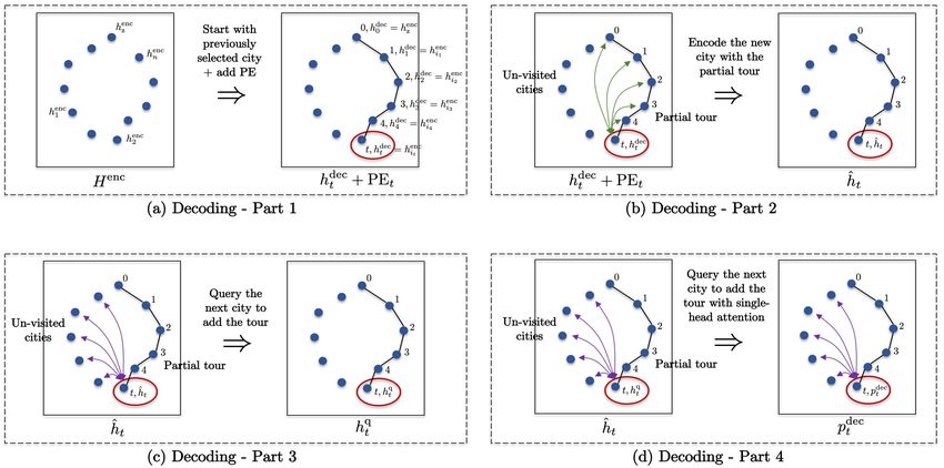
Several approximate/heuristic algorithms have been introduced. Christofides algorithm [7] approxi-
mates TSP with Minimum Spanning Trees. The algorithm has a polynomial-time complexity with
O(n2 log n), and is guaranteed to find a solution within a factor 3/2 of the optimal solution. Far-
thest/nearest/greedy insertion algorithms [20] have complexity O(n2 ), and farthest insertion (the best
insertion in practice) has an approximation ratio of 2.43. Google OR-Tools [14] is a highly optimized
program that solves TSP and a larger set of vehicle routing problems. This program applies different
heuristics s.a. Simulated Annealing, Greedy Descent, Tabu Search, to navigate in the search space,
and refines the solution by Local Search techniques. 2-Opt algorithm [27, 21] proposes an heuristic
based on a move that replaces two edges to reduce the tour length. The complexity is O(n2 m(n)),
where n2 is the number of node pairs and m(n) is the number of times all pairs must be tested to
                                                                                       √
reach a local minimum (with worst-case being O(2n/2 )). The approximation ratio is 4/ n. Extension
to 3-Opt move (replacing 3 edges) and more have been proposed in [6]. Finally, LKH-3 algorithm
[18] introduces the best heuristic for solving TSP. It is an extension of the original LKH [28] and
LKH-2 [17] based on 2-Opt/3-Opt where edge candidates are estimated with a Minimum Spanning
Tree [17]. LKH-3 can tackle various TSP-type problems.

2   Neural Network Solvers
In the last decade, Deep learning (DL) has significantly improved Computer Vision, Natural Language
Processing and Speech Recognition by replacing hand-crafted visual/text/speech features by features
learned from data [26]. For combinatorial problems, the main question is whether DL can learn better
heuristics from data than hand-crafted heuristics? This is attractive because developing algorithms
to tackle efficiently NP-hard problems require years of research (TSP has been actively studied for
seventy years). Besides, many industry problems are combinatorial. The last five years have seen the
emergence of promising techniques where (graph) neural networks have been capable to learn new
combinatorial algorithms with supervised or reinforcement learning. We briefly summarize this line
of work below.
• HopfieldNets [19]: First Neural Network designed to solve (small) TSPs.
• PointerNets [39]: A pioneer work using modern DL to tackle TSP and combinatorial optimization
problems. This work combines recurrent networks to encode the cities and decode the sequence of
nodes in the tour, with the attention mechanism. The network structure is similar to [3], which was
applied to NLP with great success. The decoding is auto-regressive and the network parameters are
learned by supervised learning with approximate TSP solutions.
• PointerNets+RL [5]: The authors improve [39] with Reinforcement Learning (RL) which eliminates
the requirement of generating TSP solutions as supervised training data. The tour length is used as
reward. Two RL approaches are studied; a standard unbiased reinforce algorithm [40], and an active
search algorithm that can explore more candidates.
• Order-invariant PointerNets+RL [33]: The original network [39] is not invariant by permutations
of the order of the input cities (which is important for NLP but not for TSP). This requires [39] to
randomly permute the input order to let the network learn this invariance. The work [33] solves this
issue by making the encoder permutation-invariant.
• S2V-DQN [9]: This model is a graph network that takes a graph and a partial tour as input, and
outputs a state-valued function Q to estimate the next node in the tour. Training is done by RL
and memory replay [31], which allows intermediate rewards that encourage farthest node insertion
heuristic.
• Quadratic Assignment Problem [34]: TSP can be formulated as a QAP, which is NP-hard and also
hard to approximate. A graph network based on the powers of adjacency matrix of node distances
is trained in supervised manner. The loss is the KL distance between the adjacency matrix of the
ground truth cycle and its network prediction. A feasible tour is computed with beam search.
• Permutation-invariant Pooling Network [23]: This work solves a variant of TSP with multiple
salesmen. The network is trained by supervised learning and outputs a fractional solution, which is
transformed into a feasible integer solution by beam search. The approach is non-autoregressive, i.e.
single pass.
• Tranformer-encoder+2-Opt heuristic [11]: The authors use a standard transformer to encode the
cities and they decode sequentially with a query composed of the last three cities in the partial
tour. The network is trained with Actor-Critic RL, and the solution is refined with a standard 2-Opt
heuristic.
• Tranformer-encoder+Attention-decoder [25]: This work also uses a standard transformer to encode

                                                  2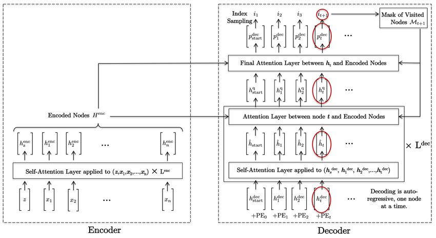
Figure 1: Proposed TSP Transformer architecture.

the cities and the decoding is sequential with a query composed of the first city, the last city in the
partial tour and a global representation of all cities. Training is carried out with reinforce and a
deterministic baseline.
• GraphConvNet [22]: This work learns a deep graph network by supervision to predict the probabili-
ties of an edge to be in the TSP tour. A feasible tour is generated by beam search. The approach uses
a single pass.
• 2-Opt Learning [41]: The authors design a transformer-based network to learn to select nodes
for the 2-Opt heuristics (original 2-Opt may require O(2n/2 ) moves before stopping). Learning is
performed by RL and actor-critic.
• GNNs with Monte Carlo Tree Search [42]: A recent work based on AlphaGo [35] which augments
a graph network with MCTS to improve the search exploration of tours by evaluating multiple next
node candidates in the tour. This improves the search exploration of auto-regressive methods, which
cannot go back once the selection of the nodes is made.

3   Proposed Architecture

We cast TSP as a “translation” problem where the source “language” is a set of 2D points and
the target “language” is a tour (sequence of indices) with minimal length, and adapt the original
Transformers [37] to solve this problem. We train by reinforcement learning, with the same setting as
[25]. The reward is the tour length and the baseline is simply updated if the train network improves
the baseline on a set of random TSPs. See Figure 1 for a description of the proposed architecture.
Encoder. It is a standard Transformer encoder with multi-head attention and residual connection. The
only difference is the use of batch normalization, instead of layer normalization. The memory/speed
complexity is O(n2 ). Formally, the encoder equations are (when considering a single head for an

                                                  3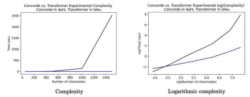
easier description)
enc
H enc = H `=L ∈ R(n+1)×d , (1)
where
H `=0 = Concat(z, X) ∈ R(n+1)×2 , z ∈ R2 , X ∈ Rn×2 , (2)
` `T
QK
H `+1 = softmax( √ )V ` ∈ R(n+1)×d , (3)
d
Q` = H ` WQ` ∈ R(n+1)×d , WQ` ∈ Rd×d , (4)
K` = H ` WK
`
∈ R(n+1)×d , WK
`
∈ Rd×d , (5)
` `
V = H WV` ∈R (n+1)×d
, WV` ∈R d×d
, (6)
(7)
where z is a start token, initialized at random. See Figure 5 for an illustration of the encoder.
Figure 2: Illustration of encoder.
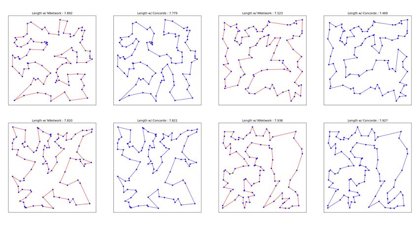
Decoder. The decoding is auto-regressive, one city at a time. Suppose we have decoded the first t
cities in the tour, and we want to predict the next city. The decoding process is composed of four
steps detailed below and illustrated on Figure 3.
Figure 3: Illustration of the four decoding steps.
Decoder – Part 1. The decoding starts with the encoding of the previously selected it city :
d
hdec
t = henc
it + PEt ∈ R , (8)
d
hdec
t=0 = hdec
start = z + PEt=0 ∈ R , (9)
4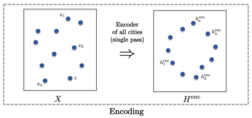
where PEt ∈ Rd is the traditional positional encoding in [37] to order the nodes in the tour:
                                                                           d
                          sin(2πfi t) if i is even,               10, 000 b2ic
             PEt,i =                                   with fi =               .                    (10)
                          cos(2πfi t) if i is odd,                     2π

Decoder – Part 2. This step prepares the query using self-attention over the partial tour. The self-
attention layer is standard and uses multi-head attention, residual connection, and layer normalization.
The memory/speed complexity is O(t) at the decoding step t. The equations for this step are (when
again considering a single head for an easier description)
                                                               T
                                                  q` K `
                     ĥ`+1
                       t         =      softmax( √ )V ` ∈ Rd , ` = 0, ..., Ldec − 1                 (11)
                                                      d
                            q`   =      ĥt Ŵq ∈ R , Ŵq` ∈ Rd×d ,
                                          `   `    d
                                                                                                    (12)
                             `            `     `             t×d        `         d×d
                        K        =      Ĥ1,t ŴK      ∈R            , ŴK    ∈R          ,         (13)
                             `            `
                        V        =      Ĥ1,t ŴV`     ∈R     t×d
                                                                     , ŴV`   ∈R   d×d
                                                                                          ,         (14)
                                                                           hdec

                       `                                                    t if ` = 0
                     Ĥ1,t       =      [ĥ`1 , .., ĥ`t ], ĥ`t =                     .            (15)
                                                                           hq,`
                                                                            t if ` > 0

Decoder – Part 3. This stage queries the next possible city among the non-visited cities using a
query-attention layer. Multi-head attention, residual connection, and layer normalization are used.
The memory/speed complexity is O(n) at each recursive step.
                                                          T
                                          q` K `
                htq,`+1      = softmax( √            Mt )V ` ∈ Rd , ` = 0, ..., Ldec − 1            (16)
                                              d
                     q`      = ĥ`+1
                                 t   W̃q` ∈ Rd , W̃q` ∈ Rd×d ,                                      (17)
                        `              enc    `          t×d  `                 d×d
                    K        =       H W̃K        ∈ R , W̃K                ∈R         ,             (18)
                        `
                    V        =       H enc W̃V`   ∈ Rt×d , W̃V`           ∈R   d×d
                                                                                     ,              (19)
                                                                                                    (20)
with Mt is the mask if the visited cities and                  is the Hadamard product.
Decoder – Part 4. This is the final step that performs a final query using a single-head attention
to get a distribution over the non-visited cities. Eventually, the next node it+1 is sampled from
the distribution using Bernoulli during training and greedy (index with maximum probability) at
inference time to evaluate the baseline. The memory/speed complexity is O(n). The final equation is
                                                            qK T
                             pdec
                              t       = softmax(C. tanh( √          Mt )) ∈ Rn ,                    (21)
                                                              d
                                 q    = hqt W̄q ∈ Rd , W̄q ∈ Rd×d ,                                 (22)
                                                enc                  n×d       `          d×d
                                 K    = H             W̄K ∈ R              , W̄K   ∈R           ,   (23)
                                                                                                    (24)
where C = 10.

4   Architecture Comparison
Comparing Transformers for NLP (translation) vs. TSP (combinatorial optimization), the order of
the input sequence is irrelevant for TSP but the order of the output sequence is coded with PEs for
both TSP and NLP. TSP-Encoder benefits from Batch Normalization as we consider all cities during
the encoding stage. TSP-Decoder works better with Layer Normalization since one vector is decoded
at a time (auto-regressive decoding as in NLP). The TSP Transformer is learned by Reinforcement
Learning, hence no TSP solutions/approximations required. Both transformers for NLP and TSP
have quadratic complexity O(n2 L).
Comparing with the closed neural network models of [25] and [11], we use the same transformer-
encoder (with BN) but our decoding architecture is different. We construct the query using all

                                                                     5
cities in the partial tour with a self-attention module. [25] use the first and last cities with a global
representation of all cities as the query for the next city. [11] define the query with the last three cities
in the partial tour. Besides, our decoding process starts differently. We add a token city z ∈ R2 . This
city does not exist and aims at starting the decoding at the best possible location by querying all cities
with a self-attention module. [25] starts the decoding with the mean representation of the encoding
cities and a random token of the first and current cities. [11] starts the decoding with a random token
of the last three cities.
5 Decoding Technique
Given a set X ∈ Rn×2 of 2-D cities, a tour is represented as an ordered sequence of city indices :
seqn = {i1 , i2 , . . . , in } and TSP can be cast as a sequence optimization problem:
max P TSP (seqn |X) = P TSP (i1 , ..., in |X). (25)
seqn ={i1 ,...,in }
For auto-regressive decoding, i.e. selecting a city one at a time, P TSP can be factorized with the chain
rule:
P TSP (i1 , ..., in |X) = P (i1 |X) · P (i2 |i1 , X) · P (i3 |i2 , i1 , X) · ... · P (in |in−1 , in−2 , ..., X). (26)
Hence the decoding problem aims at finding the sequence i1 , i2 , . . . , in that maximizes the objective:
max Πnt=1 P (it |it−1 , it−2 , ...i1 , X). (27)
i1 ,...,in
Finding exactly the optimal sequence by exhaustive search is intractable given the O(n!) complexity,
and approximations are necessary. The simplest approximate search is the greedy search; at each
time step, the next city is selected with the highest probability:
it = arg max P (i|it−1 , it−2 , ...i1 , X) (28)
i
The complexity is linear O(n).
Better sampling techniques such as beam search or Monte Carlo Tree Search (MTCS) are known to
improve results over greedy search in NLP [36] and TSP [34, 23, 25, 22, 41, 42]. Their complexity
is O(Bn), where B is the number of beams or explored paths. Beam search [29] is a breadth-first
search (BFS) technique where the breath has a limited size B. the beam search decoding problem is
as follows:
0 0
max ΠB b b b b
6 {ib1 , ..., ibn }, ∀b 6= b0
b=1 P (i1 , ..., in |X) s.t. {i1 , ..., in } = (29)
{ib1 ,...,ibn }B
b=1
For B = 1, the solution is given by greedy decoding. For B > 1, the solution at t is determined by
considering all possible extensions of B beams, and only keeping the Top-B probabilities :
n oB.(n−t)
{ib1 , ..., ibt }B
b=1 = Top-B Πtk=1 P (ibk |ibk−1 , ibk−2 , ..., ib1 , X) , (30)
b=1
or equivalently (for better numerical stabilities) :
t
nX oB.(n−t)
{ib1 , ..., ibt }B
b=1 = Top-B log P (ibk |ibk−1 , ibk−2 , ..., ib1 , X) . (31)
b=1
k=1
6 Numerical Experiments
We compare the proposed architecture with existing methods in Table 1. Our test set is composed of
10k TSP50 and TSP100. Concorde[1] run on Intel Xeon Gold 6132 CPU and the Transformers run on
Nvidia 2080Ti GPU. Our code is available on GitHub https://github.com/xbresson/TSP_Transformer.
Experimental complexity for the inference time for a single TSP is presented on Figure 4.
6TSP50 TSP100
Method Obj Gap T Time I Time Obj Gap T Time I Time
Concorde [2] 5.689 0.00% 2m* 0.05s 7.765 0.00% 3m* 0.22s
MIP
Gurobi [15] - 0.00%* 2m* - 7.765* 0.00%* 17m* -
Nearest insertion 7.00* 22.94%* 0s* - 9.68* 24.73%* 0s* -
Heuristic
Farthest insertion [20] 6.01* 5.53%* 2s* - 8.35* 7.59%* 7s* -
OR tools [14] 5.80* 1.83%* - - 7.99* 2.90%* - -
LKH-3 [18] - 0.00%* 5m* - 7.765* 0.00%* 21m* -
Vinyals et-al [39] 7.66* 34.48%* - - - - - -
Bello et-al [5] 5.95* 4.46%* - - 8.30* 6.90%* - -
Greedy Sampling
Neural Network
Dai et-al [9] 5.99* 5.16%* - - 8.31* 7.03%* - -
Deudon et-al [11] 5.81* 2.07%* - - 8.85* 13.97%* - -
Kool et-al [25] 5.80* 1.76%* 2s* - 8.12* 4.53%* 6s* -
Kool et-al [25] (our version) - - - - 8.092 4.21% - -
Joshi et-al [22] 5.87 3.10% 55s - 8.41 8.38% 6m -
Our model 5.707 0.31% 13.7s 0.07s 7.875 1.42% 4.6s 0.12s
Kool et-al [25] (B=1280) 5.73* 0.52%* 24m* - 7.94* 2.26%* 1h* -
Kool et-al [25] (B=5000) 5.72* 0.47%* 2h* - 7.93* 2.18%* 5.5h* -
Advanced Sampling
Joshi et-al [22] (B=1280) 5.70 0.01% 18m - 7.87 1.39% 40m -
Neural Network
Xing et-al [42] (B=1200) - 0.20%* - 3.5s* - 1.04%* - 27.6s*
Wu et-al [41] (B=1000) 5.74* 0.83%* 16m* - 8.01* 3.24%* 25m* -
Wu et-al [41] (B=3000) 5.71* 0.34%* 45m* - 7.91* 1.85%* 1.5h* -
Wu et-al [41] (B=5000) 5.70* 0.20%* 1.5h* - 7.87* 1.42%* 2h* -
Our model (B=100) 5.692 0.04% 2.3m 0.09s 7.818 0.68% 4m 0.16s
Our model (B=1000) 5.690 0.01% 17.8m 0.15s 7.800 0.46% 35m 0.27s
Our model (B=2500) 5.689 4e-3% 44.8m 0.33s 7.795 0.39% 1.5h 0.62s
Table 1: Comparison with existing methods. Results with * are reported from other papers. T Time
means total time for 10k TSP (in parallel). I Time means inference time to run a single TSP (in
serial).
Figure 4: Experimental complexity.
7 Discussion
In this work, we essentially focused on the architecture. We observe that the Transformer architecture
can be successful to solve the TSP Combinatorial Optimization problem, expanding the success
of Transformer for NLP and CV. It also improves recent learned heuristics with an optimal gap of
0.004% for TSP50 and 0.39% for TSP100.
Further developments can be considered with better sampling techniques such as group beam-search
[38, 30] or MCTS [42] which are known to improve results. Besides, the use of heuristics like 2-Opt
to get intermediate rewards has also shown improvements [41] (the tour length as global reward
requires to wait the end of the tour construction).
However, traditional solvers like Concorde/LKH-3 still outperform learning solvers in terms of
performance and generalization, although neural network solvers offer faster inference time, O(n2 L)
vs. O(n2.5 b(n)), where O(b(n)) is the number of branches to explore in BB.
What’s next? The natural next step is to scale to larger TSP sizes for n > 100 but it is challenging as
GPU memories are limited, and Transformer architectures and auto-regressive decoding are in O(n2 ).
7Figure 5: Visualization of TSP100 instances.
We could consider “harder” TSP/routing problems where traditional solvers like Gurobi/LKH-3 can
only provide weaker solutions or would take very long to solve. We could also work on “harder”
combinatorial problems where traditional solvers s.a. Gurobi cannot be used.
Another attractive research direction is to leverage learning techniques to improve traditional solvers.
For example, traditional solvers leverage Branch-and-Bound technique [4, 16]. Selecting the variables
to branch is critical for search efficiency, and relies on human-engineered heuristics s.a. Strong
Branching [1] which is a high-quality but expensive branching rule. Recent works [13, 32] have
shown that neural networks can be successfully used to imitate expert heuristics and speed-up the BB
computational time. Future work may focus on going beyond imitation of human-based heuristics,
and learning novel heuristics for faster Branch-and-Bound technique.
8 Conclusion
The field of Combinatorial Optimization is pushing the limit of deep learning. Traditional solvers still
provide better solutions than learning models. However, traditional solvers have been studied since
the 1950s and the interest of applying deep learning to combinatorial optimization has just started.
This topic of research will naturally expend in the coming years as combinatorial problems problems
s.a. assignment, routing, planning, scheduling are used every day by companies. Novel software may
also be developed that combine continuous, discrete optimization and learning techniques.
9 Acknowledgement
Xavier Bresson is supported by NRF Fellowship NRFF2017-10.
References
[1] Tobias Achterberg, Thorsten Koch, and Alexander Martin. 2005. Branching rules revisited.
Operations Research Letters 33, 1 (2005), 42–54.
[2] David L Applegate, Robert E Bixby, Vasek Chvatal, and William J Cook. 2006. The traveling
salesman problem: a computational study. Princeton university press.
[3] Dzmitry Bahdanau, Kyunghyun Cho, and Yoshua Bengio. 2014. Neural machine translation by
jointly learning to align and translate. arXiv preprint arXiv:1409.0473 (2014).
8[4] Richard Bellman. 1962. Dynamic programming treatment of the travelling salesman problem.
Journal of the ACM (JACM) 9, 1 (1962), 61–63.
[5] Irwan Bello, Hieu Pham, Quoc V Le, Mohammad Norouzi, and Samy Bengio. 2016. Neural
combinatorial optimization with reinforcement learning. arXiv preprint arXiv:1611.09940
(2016).
[6] Andrius Blazinskas and Alfonsas Misevicius. 2011. combining 2-opt, 3-opt and 4-opt with
k-swap-kick perturbations for the traveling salesman problem. Kaunas University of Technology,
Department of Multimedia Engineering, Studentu St (2011), 50–401.
[7] Nicos Christofides. 1976. Worst-case analysis of a new heuristic for the travelling sales-
man problem. Technical Report. Carnegie-Mellon Univ Pittsburgh Pa Management Sciences
Research Group.
[8] Georges A Croes. 1958. A method for solving traveling-salesman problems. Operations
research 6, 6 (1958), 791–812.
[9] Hanjun Dai, Elias B Khalil, Yuyu Zhang, Bistra Dilkina, and Le Song. 2017. Learning
combinatorial optimization algorithms over graphs. arXiv preprint arXiv:1704.01665 (2017).
[10] George Dantzig, Ray Fulkerson, and Selmer Johnson. 1954. Solution of a large-scale traveling-
salesman problem. Journal of the operations research society of America 2, 4 (1954), 393–410.
[11] Michel Deudon, Pierre Cournut, Alexandre Lacoste, Yossiri Adulyasak, and Louis-Martin
Rousseau. 2018. Learning heuristics for the tsp by policy gradient. In International conference
on the integration of constraint programming, artificial intelligence, and operations research.
Springer, 170–181.
[12] Marshall L Fisher. 1981. The Lagrangian relaxation method for solving integer programming
problems. Management science 27, 1 (1981), 1–18.
[13] Maxime Gasse, Didier Chételat, Nicola Ferroni, Laurent Charlin, and Andrea Lodi. 2019. Exact
Combinatorial Optimization with Graph Convolutional Neural Networks. In Advances in Neural
Information Processing Systems, Hanna M. Wallach, Hugo Larochelle, Alina Beygelzimer,
Florence d’Alché-Buc, Emily B. Fox, and Roman Garnett (Eds.). 15554–15566.
[14] Google. 2015. OR-tools: Google’s Operations Research tools.
[15] Z Gu, E Rothberg, and R Bixby. 2008. Gurobi.
[16] Michael Held and Richard M Karp. 1962. A dynamic programming approach to sequencing
problems. Journal of the Society for Industrial and Applied mathematics 10, 1 (1962), 196–210.
[17] Keld Helsgaun. 2000. An effective implementation of the Lin–Kernighan traveling salesman
heuristic. European Journal of Operational Research 126, 1 (2000), 106–130.
[18] Keld Helsgaun. 2017. An extension of the Lin-Kernighan-Helsgaun TSP solver for constrained
traveling salesman and vehicle routing problems. Roskilde: Roskilde University (2017).
[19] John J Hopfield and David W Tank. 1985. “Neural” computation of decisions in optimization
problems. Biological cybernetics 52, 3 (1985), 141–152.
[20] David S Johnson. 1990. Local optimization and the traveling salesman problem. In International
colloquium on automata, languages, and programming. Springer, 446–461.
[21] S Johnson David and A McGeoch Lyle. 1995. The Travelling Saleman Problem: A case study
in Local Optimization. AT&T Labs, Florham Park, Department of Mathematics and Computer
Science, Amherst College (1995).
[22] Chaitanya K Joshi, Thomas Laurent, and Xavier Bresson. 2019. An efficient graph convolutional
network technique for the travelling salesman problem. arXiv preprint arXiv:1906.01227
(2019).
9[23] Yoav Kaempfer and Lior Wolf. 2018. Learning the multiple traveling salesmen problem with
permutation invariant pooling networks. arXiv preprint arXiv:1803.09621 (2018).
[24] Scott Kirkpatrick, C Daniel Gelatt, and Mario P Vecchi. 1983. Optimization by simulated
annealing. science 220, 4598 (1983), 671–680.
[25] Wouter Kool, Herke Van Hoof, and Max Welling. 2018. Attention, learn to solve routing
problems! arXiv preprint arXiv:1803.08475 (2018).
[26] Yann LeCun, Yoshua Bengio, and Geoffrey Hinton. 2015. Deep learning. nature 521, 7553
(2015), 436–444.
[27] Shen Lin. 1965. Computer solutions of the traveling salesman problem. Bell System Technical
Journal 44, 10 (1965), 2245–2269.
[28] Shen Lin and Brian W Kernighan. 1973. An effective heuristic algorithm for the traveling-
salesman problem. Operations research 21, 2 (1973), 498–516.
[29] Bruce T Lowerre. 1976. The HARPY speech recognition system. Ph. D. Thesis (1976).
[30] Clara Meister, Tim Vieira, and Ryan Cotterell. 2020. Best-first beam search. Transactions of
the Association for Computational Linguistics 8 (2020), 795–809.
[31] Volodymyr Mnih, Koray Kavukcuoglu, David Silver, Alex Graves, Ioannis Antonoglou, Daan
Wierstra, and Martin Riedmiller. 2013. Playing atari with deep reinforcement learning. arXiv
preprint arXiv:1312.5602 (2013).
[32] Vinod Nair, Sergey Bartunov, Felix Gimeno, Ingrid von Glehn, Pawel Lichocki, Ivan Lobov,
Brendan O’Donoghue, Nicolas Sonnerat, Christian Tjandraatmadja, Pengming Wang, Ravichan-
dra Addanki, Tharindi Hapuarachchi, Thomas Keck, James Keeling, Pushmeet Kohli, Ira Ktena,
Yujia Li, Oriol Vinyals, and Yori Zwols. 2020. Solving Mixed Integer Programs Using Neural
Networks. CoRR abs/2012.13349 (2020).
[33] Mohammadreza Nazari, Afshin Oroojlooy, Lawrence V Snyder, and Martin Takáč. 2018. Rein-
forcement learning for solving the vehicle routing problem. arXiv preprint arXiv:1802.04240
(2018).
[34] Alex Nowak, Soledad Villar, Afonso S Bandeira, and Joan Bruna. 2017. A note on learning
algorithms for quadratic assignment with graph neural networks. stat 1050 (2017), 22.
[35] David Silver, Aja Huang, Chris J Maddison, Arthur Guez, Laurent Sifre, George Van Den Driess-
che, Julian Schrittwieser, Ioannis Antonoglou, Veda Panneershelvam, Marc Lanctot, et al. 2016.
Mastering the game of Go with deep neural networks and tree search. nature 529, 7587 (2016),
484–489.
[36] Christoph Tillmann and Hermann Ney. 2003. Word reordering and a dynamic programming
beam search algorithm for statistical machine translation. Computational linguistics 29, 1
(2003), 97–133.
[37] Ashish Vaswani, Noam Shazeer, Niki Parmar, Jakob Uszkoreit, Llion Jones, Aidan N Gomez,
Lukasz Kaiser, and Illia Polosukhin. 2017. Attention is all you need. arXiv preprint
arXiv:1706.03762 (2017).
[38] Ashwin K Vijayakumar, Michael Cogswell, Ramprasath R Selvaraju, Qing Sun, Stefan Lee,
David Crandall, and Dhruv Batra. 2016. Diverse beam search: Decoding diverse solutions from
neural sequence models. arXiv preprint arXiv:1610.02424 (2016).
[39] Oriol Vinyals, Meire Fortunato, and Navdeep Jaitly. 2015. Pointer networks. arXiv preprint
arXiv:1506.03134 (2015).
[40] Ronald J Williams. 1992. Simple statistical gradient-following algorithms for connectionist
reinforcement learning. Machine learning 8, 3-4 (1992), 229–256.
[41] Yaoxin Wu, Wen Song, Zhiguang Cao, Jie Zhang, and Andrew Lim. 2019. Learning improve-
ment heuristics for solving routing problems. arXiv preprint arXiv:1912.05784 (2019).
[42] Zhihao Xing and Shikui Tu. 2020. A graph neural network assisted Monte Carlo tree search
approach to traveling salesman problem. IEEE Access 8 (2020), 108418–108428.
10You can also read