Contact-free measurement and numerical and analytical evaluation of the strain distribution in a wood-FRP lap-joint
←
→
Page content transcription
If your browser does not render page correctly, please read the page content below
Materials and Structures
DOI 10.1617/s11527-009-9568-x

 ORIGINAL ARTICLE

Contact-free measurement and numerical and analytical
evaluation of the strain distribution in a wood-FRP lap-joint
Johan Vessby • Erik Serrano • Bertil Enquist

Received: 8 May 2009 / Accepted: 26 November 2009
Ó RILEM 2009

Abstract Wood specimens to each of which a                      anchorage length in a non-linear fashion. The exper-
laminate of carbon fibre reinforcement polymers                 imental, analytical and numerical results were shown
(FRP) was glued (creating a lap joint in each case)             to be in close agreement with respect to the strength
were loaded to failure. A total of 15 specimens of              and the strain distribution obtained.
three types differing in the glued length (anchorage
length) of the FRP laminate (50, 150 and 250 mm                 Keywords     FRP  Lap-joint  Volkersen  Wood
respectively) were tested, their strength, stiffness and
strain distribution being evaluated. Synchronized
digital cameras (charge-coupled devices) used in                1 Background
testing enabled strain fields on surfaces they were
directed at during the loading procedure to be                  In the building sector, enhancement of the load-
measured. These results were also evaluated both                carrying capacity of new or already existing structures
analytically on the basis of generalized Volkersen              without any change in their geometry needing to be
theory and numerically by use of the finite element             made may be sought. This may be based on changed
method. The lap joints showed a high level of                   conditions, such as an increase in loading due to
stiffness as compared with mechanical joints. A high            rebuilding or redesigning of the overall structure.
degree of accuracy in the evaluation of stiffness was           Points in close proximity to connections between
achieved through the use of the contact-free evalu-             different building elements or around holes or notches
ation system. The load-bearing capacity of joints of            in beams, for example, can be in particular need
this type was found to be dependent upon the                    of reinforcement. What is aimed at may be greater
                                                                stiffness, enhanced load-bearing capacity, or both.
                                                                One method of increasing the stiffness and strength of
J. Vessby                                                       a structure is by use of Fibre Reinforced Polymers
Tyréns, Storgatan 40, 352 31 Växjö, Sweden                   (FRP). These show a very high level of strength and
                                                                stiffness as compared with many other materials.
J. Vessby (&)  E. Serrano  B. Enquist
Växjö University, Lückligs Plats 1, 351 95 Växjö, Sweden       The aim of the present study was to investigate
e-mail: johan.vessby@vxu.se                                     experimentally under well-defined conditions and
E. Serrano                                                      evaluate analytically and numerically the properties
e-mail: erik.serrano@vxu.se                                     of the interaction between FRP-laminates (referred to
B. Enquist                                                      hereafter as FRPs) and timber to which they are glued
e-mail: bertil.enquist@vxu.se                                   to form single-overlap joints (these are also termed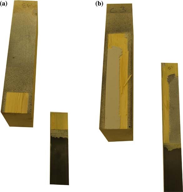
Materials and Structures

lap-joints). Other researchers, such as Gustafsson and
                                                                      [mm]
Enquist [1], Johansson et al. [2] and Kliger et al. [3]
have reported both experimentally and numerically                                                        Indicates the fibre
based findings concerning properties of the FRP-                                    145                orientation of the wood
timber interaction. In these studies no use was made of                  70                            and FRP respectively.
a contact-free evaluation system to examine in detail      Wood
                                                                                                  350
the behaviour of the joint, a matter the very large
amount of data obtained by use of such a system makes        FRP
possible. Guan et al. [4] studied a timber beam                                                       Part of the timber where

reinforced with glass fibre pretensioned to different                                                 m.c. was evaluated after test.
forces. They compared the load–deflection relations           lglue
between a three-dimensional finite element model and                    50     10

experimental results and obtained good agreement.                                           y

   One can note that experiments have also been
performed with the aim of developing design equa-                                                 x
                                                                                       z
tions for glued-in rods, an application that shows
strong similarities to FRP overlap joints, see Steiger                 t=1.4        150 + lglue
et al. [5, 6]. In the present study no design parameters
are proposed. The objective is rather to investigate
the usefulness of various methods for analyzing FRP        Fig. 1 The test specimens, 70 9 145 mm2 in cross section,
lap joints. One of these is the contact-free evaluation    were sawn to 350 mm in length. The FRP was glued to them
system just referred to. Two others are the use of         using three different anchorage lengths (lglue): 50, 150 and
                                                           250 mm
analytical models based on generalized Volkersen
theory (see [7, 8]), and analysis by use of the finite
element method.                                            by means of a spatula. Each FRP was centrically
                                                           placed on one edge of the wood specimen in question,
                                                           such that there was 10 mm clearance to the edge of
2 Materials and methods                                    the specimen, see Fig. 1. No clamping was used
                                                           while attaching the two pieces to each other.
2.1 Test specimens                                            The specimens were of three different types, A, B
                                                           and C, differing in the length of the overlap, lglue,
Wooden test specimens of Norway Spruce 350 mm              such that the specimens in the groups had a glued
in length were sawn from 5 m long boards 70 9              overlap of 50, 150 and 250 mm, respectively. After
145 mm2 in cross-section. Prior to any further han-        the FRP had been glued to the wood, the specimens
dling, the wood specimens were stored in a standard        were once again stored in the 20°C/65% standard
climate at 20°C and a relative humidity of 65% until       climate. For each of the three groups, five test
moisture equilibrium was achieved. After completion        specimens were manufactured, enabling 15 tests to be
of the experiments, conducted thereafter, the moisture     performed. The part of the FRP sticking out from the
content of the wood specimens was verified by oven         piece of wood to which it was attached was 150 mm
drying and then weighting them. Just prior to the          in length in each case. This part of the FRP was used
experiments, the surface on the side on which the FRP      for applying loads by means of the hydraulic grip of
was to be attached by glue was planed.                     the testing machine.
   The FRPs were 1.4 mm thick their stiffness and
strength, as stated by the manufacturer, were 150 and      2.2 Experimental setup
2000 MPa respectively. All carbon fibres where
oriented in the same direction. The FRPs were glued        The experimental setup, cf. Fig. 2, aimed at trans-
to the wood by use of a 2-component epoxy adhesive         mitting shear forces within the plane between the
(Resin 220) using an amount of adhesive producing a        FRP and the timber. The specimen was fixed on its
bond line thickness of 1.3 mm. The glue was applied        upper end-grain surface by means of a short steel
Materials and Structures

                                                             displacement of the piston and utilizing a contact-free
                                                             measurement system (AramisTM). An obvious differ-
                                                             ence between the two deformation measurement
  Grip and
loading point
                                                             methods is that measurements of piston displacement
                                                             are affected by the flexibility of the setup as a whole
  Top beam
                                                             and of the test specimen itself, whereas using the
                                                             contact-free system displacements between any two
 Analysis area                                               points within the field of measurements can be
for the contact-                                             determined. This latter technique enables the entire
  free system                                                field of in-plane strains to be measured continuously
                                                             in the course of an experiment.
                                                                The contact-free measurement technique is based
  Steel plate                                                on the use of two cameras which are placed in front
                                                             of the test object at angles and distances determined
                                                             by the size of the object and by the lenses involved.
                                                             With the two cameras, a number of stereoscopic
                                                             pictures are obtained during testing. The current 3D
Fig. 2 Experimental setup. Testing machine. The area eval-   position of any point within the measurement field
uated by means of the contact-free measurement system is     can then be determined by post processing the
indicated
                                                             pictures using the software being a part of the
beam having dimensions of 50 9 50 mm2. The beam              measurement system. A spray-painted, randomly
was held in place and in contact with the specimen by        distributed black and white pattern on the surface of
use of tie-down threaded rods of the M20 type,               the test object, deforming along with the test object
together with a washer and a nut. The tie-down rods          itself during loading, enables the in-plane strains to
were anchored to a solid steel structure (a part of the      be assessed. Post-processing of the pictures starts
testing machine). The load was applied at the free end       with identification of a reference state, here being that
of the FRP by displacement-controlled movement,              of the unloaded specimen. Each picture is then
the displacement increasing successively at 0.5 mm/          subdivided into partially overlapping sections, or
min. The loading rate was adjusted so as to lead to          facets, the size and amount of overlap being set by
failure of the specimen within 1–3 min. The load cell        the user on the basis of the spatial resolution and
employed had a capacity of 100 kN and a linear               accuracy desired. The gray-scale of the pictures is
tolerance interval of ±0.1%. An overview of the              utilized in performing cross-correlation calculations,
setup is shown in Fig. 3.                                    such that each facet position can be tracked with sub-
                                                             pixel accuracy from one pair of pictures to the next.
2.3 Collection of experimental data                          This allows different strain measures pertaining from
                                                             the displacement field to be calculated.
Along with registering the force applied by the                 The frame-grabbing intervals of the two cameras
testing machine, deformation data was collected              were adjusted so that 50–100 pictures per camera
using two different methods: measuring the vertical          were obtained during each test. The sampling of the

Fig. 3 Overview of the test
setup and the data collection                                                                     Control board for the
                                      Load cell ± 100 kN                                          MTS- system.
system

                                 Volume in which the test
                                 specimen is to be placed.                                        CCD- cameras connected
                                                                                                  to a data-collection and
                                                                                                  evaluation system.
Materials and Structures

load and displacement signals from the testing                   adhesive layer, b is the width of the adhesive layer, E
machine was synchronized in time with the pictures               is the modulus of elasticity, and A is the equivalent
taken.                                                           area in the wood and in the FRPs respectively. The
                                                                 general solution to the differential equation (1) is
2.4 Analytical analysis
                                                                 sð yÞ ¼ C1 coshðxyÞ þ C2 sinhðxyÞ þ sp                   ð3Þ
Analytical models for interaction between wood and               The constants C1 and C2 can be calculated using the
FRP involving different boundary conditions can be               boundary conditions, which for the present case are
formulated. A detailed account of how this can be                N1(0) = P, N2(0) = -P, N1(L) = 0 and N2(L) = 0.
done by use of the generalized Volkersen theory, as it           These conditions enable an expression of shear stress,
is called, is given by Serrano and Gustafsson [7]. As            s(y), to be obtained:
shown by e.g. Kirlin [9], the state of stress in the
                                                                          Px coshðxyÞ
overlap joint can be mulitaxial. For example stresses            sð y Þ ¼               sinhðxyÞ                  ð4Þ
                                                                           b tanhðxLÞ
perpendicular to the loading direction (peel direction)
could develop close to the end of the FRP strip. Such            This expression can be used to obtain the force N1 by
stresses can, in general, be assumed to influence the            integration of the shear stress times the width b.
level at which failure is initiated, but also the ultimate
                                                                                           sinhðxyÞ
load level. The generalized Volkersen theory used                N1 ð yÞ ¼ P coshðxyÞ                              ð5Þ
here includes only longitudinal shear, although also                                      tanhðxLÞ
peel stress could be included in the analysis, for               The corresponding strains in the FRP are found to be
example by including the shear deformation of the
wood, see Gustafsson and Serrano [10]. In order to                         N1 ð yÞ    P                 sinhðxyÞ
                                                                 e1 ð yÞ ¼         ¼         coshðxyÞ             ð6Þ
keep the analytical expression as simple as possible,                      E1 A1     E1 A 1             tanhðxLÞ
the 1D-theory is used here, however.                             This expression implies that, for any given values of
   Definitions of the symbols used in defining the               the load P and of the anchorage length L, the strains
specimen and the boundary conditions in question are             in the FRP, e1, within the interval 0 B y B L can be
shown in Fig. 4.                                                 obtained.
   In the conventional Volkersen theory, [8], the                   The expressions above are for linear elastic
differential equation for the shear stress present in a          materials. The so-called generalized Volkersen the-
lap joint can be expressed as                                    ory, [7], enables the fracture energy of the bond-line
s00  x2 s ¼ 0                                        ð1Þ        to be introduced as an additional parameter. This is
                                                                 done by introducing the equivalentshear stiffness of
where                                                            the adhesive layer. Accordingly, s2f ð2Gf Þ rather than
                                                               G/t is used to determine the shear stiffness, where Gf
  2 Gb   1     1
x ¼         þ                                         ð2Þ        is the fracture energy of the bond line and sf is the
     t E2 A2 E 1 A1
                                                                 intrinsic shear strength of the bond line. Introducing
In the expressions above, G is the shear stiffness of            the equivalent shear stiffness into (1)–(4) and
the adhesive layer, t represents the thickness of the            assuming that the joint fails when the maximum

Fig. 4 Definitions of                                             y=0                     y=L                      y
parameters used in the
                                      P         FRP      1
analytical equations
                                                                                                t1

                                                             P             Thickness of              WOOD      2            t2
                                                                           glue: t
Materials and Structures
stress at the most stressed point in the bond line Table 1 Material parameters used in the finite element
equals sf allows an expression for the normalized analyses
strength of the lap joint to be derived: Material MOE Poissons ratio
Pf tanhðxlÞ Wood 10 GPa 0.3
¼ ð7Þ
Asf xl Epoxy, Resin 220 62 MPa a
0.2
where A is the area of the overlap (i.e. A = b 9 lglue). FRP 150 GPa 0.1
For ductile joints, i.e. those in which x approaches a
Pertains to the calculated equivalent modulus of elasticity
zero, the normalized strength equals unity. This
means, in turn, that for such joints the shear stress
distribution is uniform. Consequently, the governing since they include possible interface effects in the
material parameter for prediction of the load bearing layers between the glue and the wood and between the
capacity is the local strength of the bond line, sf. glue and the FRP. In order to keep the model as small as
When x is sufficiently large (approaching infinity), possible with respect to the number of degrees of
the corresponding ‘‘strength’’ parameter governing freedom, account is taken of the symmetry of the test
the load-bearing capacity of the joint is the fracture set-up. The finite element model was loaded by
energy of the bond line. Under such conditions, the displacement-controlled movement, the same way that
prediction of (7) yields the same result as that it was done in the experiment. The boundary conditions
provided by classical linear-elastic fracture mechan- used in the finite element model are shown in Fig. 5.
ics theory (LEFM), and the load bearing capacity is Since the main purpose of the current FE-analyses was
e.g. independent of the glued length l, but depends on to visualize the general stress distribution along the
the ratio of the adherend axial stiffnesses, E1A1/ FRP, and not to estimate a single point maximum stress
(E2A2). In cases between the two extreme cases value at e.g. the corners of the FRP, no mesh refinement
above, both the local strength and the fracture energy was used in the FE-models.
influence the load-bearing capacity of the joint. Thus,
the generalized Volkersen theory can be said to be a
unifying theory. 3 Results and discussion
2.5 Analysis using the finite element method 3.1 Strength
The test specimens were also analyzed numerically The load-bearing capacities obtained from the exper-
using the finite element method. Similar analyses iments of each of the fifteen specimens that were
have been carried out by Serrano [11], for example, tested, together with the average value obtained for
with use of nonlinear FEM. A numerical and each of the three groups, are shown in Table 2. The
experimental study of glued-in rods in which strain average value for groups A, B and C i.e. for anchorage
distributions similar to those achieved in the present lengths 50, 150 and 250 mm, were 18.4, 32.8 and
study has been carried out by del Senno et al. [12]. 35.5 kN, respectively. This shows clearly that the
In order to perform the present analysis six material load-bearing capacity depends on the anchorage
parameters, two for each material, were introduced length, although in a non-linear fashion, and that
under the assumption of the material being linear- the influence of the anchorage length diminishes as
elastic isotropic, see Table 1. This is obviously an the anchorage length increases. The highest load-
approximation since wood, for example, is normally bearing capacity was that obtained for group C, which
considered to be a strongly orthotropic material, yet for had the greatest anchorage length, however in group
the analysis here the approximation is quite adequate, B, having an anchorage length 40% less, the strength
since the load is introduced primarily in the longitu- is only 7.6% lower. In addition, in group A the
dinal direction of the wood. The accuracy of the anchorage length is 20% that of the anchorage length
FE-model was verified by use of models involving in group C, whereas the load-bearing capacity for that
orthotropic parameters. The properties that are given group is nearly 50% of that obtained for group C. In
for the glue should be considered as equivalent values Fig. 6 the average strength is shown as a functionMaterials and Structures
Fig. 5 Boundary B.C. used in the FE- analysis.
conditions and loading of [mm]
the finite element model Front view Side view
used for simulation of the
lap-joint
145
70
Wood 350
FRP
lglue
50
150 + lglue
t=1.4 Displacement controlled
loading.
40
Table 2 Load-bearing capacities obtained for specimens
within groups A, B and C and the mean value for each group 35
Group A B C
30
Average strength [kN]
Anchorage length 50 mm 150 mm 250 mm
25
Test specimen
1 16.9 31.5 33.7 20
2 20.3 36.9 36.6
15
3 16.4 31.9 36.5
4 18.8 32.4 35.5 10
5 19.4 31.1 35.4 5
Average load-bearing capacity 18.4 32.8 35.5
0
The values are given in kN 0 50 100 150 200 250 300
Anchorage length [mm]
of the anchorage length, highlighting the highly Fig. 6 Average of experimentally obtained results for anchor-
non-linear nature of this relation. age lengths 50, 150 and 250 mm respectively
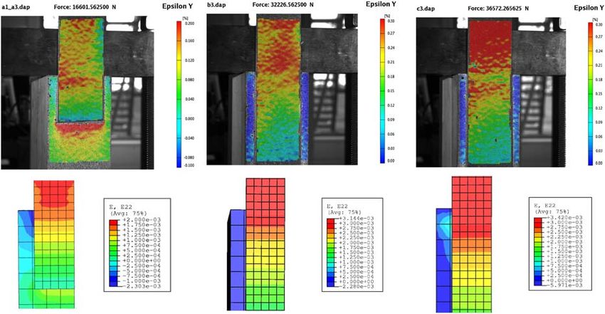
Two different failure modes were found to occur
in the experiment, one of these being shear failure of The normalized strength of a joint as a function of
the wood material and the other a combination of the anchorage length is shown in Fig. 8. The analytical
failure of the wood and of the adhesive at the solution has been fitted to the experimentally obtained
interface between the FRP and glue. An example of result in a least square sense, by varying the shear
each of these two modes is shown in Fig. 7. Most strength sf and the fracture energy Gf. The fit to the
common for all three different anchorage lengths was analytical solution yielded a value of 8.2 MPa for
the shear failure of the wood material. the shear strength and 1700 Nm/m2 for the fractureMaterials and Structures
Fig. 7 An example of each
of the two failure modes
that appeared: a shear
failure of the wood material
(test specimen A3),
b combination of shear
failure of the wood and
adhesive failure at the
junction of wood fibre and
epoxy (test specimen C3)
joint for shorter than for longer anchorage lengths. The
1
shape of the curve follows closely the three mean
results of the experiments. Note that more experiments
Normalized strength [-]
0.8
should be performed in order to verify the curve for
longer anchorage lengths, those longer than around
0.6 300 mm. The results agree well with results previously
obtained by e.g. Johansson et al. [2] and Steiger et al.
0.4 [5].
0.2
3.2 Stiffness
0 Figure 9 shows the load–displacement response
0 50 100 150 200 250 300 350 400
Anchorage length [mm] obtained in the tests. Curves based on displacement
as measured by the vertical displacement of the
Fig. 8 Normalized strength of the joint as a function of the piston and as well as curves based on displacement as
anchorage length. The analytical expression (8) is shown as a
measured by the contact-free system are shown.
solid line and the measured normalized strength for each of the
three groups A, B and C is marked with an asterisk Using the curves based on the vertical displacement
of the piston, the stiffness can be calculated to be
energy. The effective area in the wood was assumed to approximately 30 MN/m. This value is independent
be 50 mm wide and 50 mm deep, as based on the width of the anchorage length. The differences between the
of the FRP and the depth of the top beam. The curve plotted curves can be partly explained in terms of
shows a given change in anchorage length to have a local phenomena in the test setup. In the curves based
stronger influence on the normalized strength of the on the vertical movement of the piston those effectsMaterials and Structures
Fig. 9 Load–displacement 40
curves for all 15 specimens
when the vertical 35
displacement is measured in
the piston and for eight of 30
the specimens when the
vertical displacement is 25
Load [kN]
obtained from the contact-
free (c-f) system 20
15 A1 A2 A3 A4
A5 B1 B2 B3
10 B4 B5 C1 C2
C3 C4 C5 A1 c-f
5 A2 c-f A3 c-f B1 c-f B2 c-f
B3 c-f C2 c-f C3 c-f
0
0 0,5 1 1,5 2
Displacement [mm]
vertical displacement from vertical displacement
the contact-free system from the piston
will be included in contradiction to the curves based
on the contact-free system. FRP
In order to avoid inclusion of the flexibility of the
test set-up in measuring the lap-joint stiffness, test
specimen numbers 1, 2 and 3 in each group were [mm]
evaluated with respect to the relative vertical dis- P2
placement between a point P1 located on the piece of ~10
P1
wood 10 mm from the upper edge and a point P2 35
located in the center of the FRP on the edge of the
wood piece, see Fig. 10. This was easily done by 25
use of the optical evaluation system. The relation
between the load and this relative displacement, y
together with the load and vertical displacements as
obtained from the piston, are shown in Fig. 9. For the
case in which the distance between the two points is Line 1
employed, the stiffness obtained is about 180 kN/m,
some six times as high as when the vertical position x
of the piston is the basis for the calculations. This WOOD
difference highlights the power of using an optical
system with the possibilities it provides of selecting
Fig. 10 Definitions of points P1 and P2 between which
evaluation points after testing has been performed.
vertical displacements were measured, and Line 1, along
The accuracy of testing can be markedly increased in which the strain component ey was measured
this way.
of the three cases shows the results obtained for a
3.3 Strain distribution given load from the contact-free system, the bottom
part of the respective figure showing the results of the
It can be shown from results obtained using the finite element analysis for the same load. The red
contact-free system how the strain (ey) varies over a colour indicates large strains and the blue colour
given specimen. Figure 11 presents an example from small to negative strains. It can be readily seen that
each of the three groups of how strain is distributed in the strains in the FRP are largest close to the edge of
a test specimen. The upper part of the figure in each the piece of wood, their decreasing then toward in theMaterials and Structures
Fig. 11 Examples of strains ey close to failure obtained in one of the testings in each of the three groups. ey for a test specimen from
group A, F = 16.6 kN; ey for a test specimen from group B, F = 32.2 kN; ey for a test specimen from group C, F = 36.6 kN
inner parts of the glued area. For group A it can also maximum strain just prior to failure was 1.45% for
be seen that the strains are largest in the part of the group A, 2.80% for group B and 2.81% for group C.
wood toward the end of the FRP. The figure shows that the normal strains (in the
In Fig. 12 the normal strains in the FRP along line FRP) at the edge are appreciably lower in group A
1, defined as in Fig. 10, obtained in three different than in groups B and C, where they are quite similar
ways are compared with each other for group A, B in size. The relatively linear strain distribution can be
and C respectively. The strains shown are those explained by the fact that the glue is of relatively low
obtained by use of the contact-free measurement stiffness compared with the material it is glued to. A
system, as well as on the basis of the analytical perfectly linear distribution would imply that the
expression and the numerical FE-analysis. The strains shear stress in the bond line is constant along the
obtained in the experiments were averaged within overlap. The analytical calculations, as previously
each group before being plotted in the figure. The indicated, are based for each of the specimens on an
Fig. 12 Moving average of 4,00
the component ey in the FRP Grupp A - experimental
at maximum load within Grupp B - experimental
each group. The analytical 3,00 Grupp C - experimental
results and the results of the Grupp A - analytical
Milli strain [-]
finite element analysis are Grupp B - analytical
also shown for each of the Grupp C - analytical
2,00
three groups Grupp A - FEM
Grupp B - FEM
Grupp C - FEM
1,00
0,00
0 20 40 60 80 100 120 140 160 180 200 220 240
Anchorage length [mm]Materials and Structures
effective area of 50 9 50 mm2 and a glue thickness – The load-bearing capacity of the joint is partly a
of t = 1.3 mm. The equivalent shear modulus G of function of the anchorage length, becoming
the glue can be calculated as having a value of greater if the anchorage length is increased, but
25.7 MPa according to the formula beyond a certain point the anchorage length
appears to play only a limited role. In the
s2f t
G¼ ð8Þ experiments carried out, this was shown by the
2Gf fact that, despite there being about a 40%
where the shear strength sf = 8.2 MPa and the difference in anchorage length between groups
fracture energy Gf = 1700 Nm/m2. The results of B and C, the average strength of the two differed
the three-dimensional FE-analysis are also shown in by only about 10%.
Fig. 12. A thickness of t = 1.3 mm was used for the – The strain was found to be at a maximum at a
glue, the corresponding modulus of elasticity being point close to the end of the piece of wood. The
calculated as 62 MPa (corresponding to a G = maximum strain measured prior to failure was
25.7 MPa and a Poisson’s ratio of m = 0.2). The 1.45% for group A, 2.80% for group B and
agreement between the calculations and the results of 2.81% for group C (average values).
the experiments is rather close, implying that calcula- – For the type of lap-joints involved, close agree-
tions for the type of lap joints shown here can be done ment between results of the experiments and
analytically using generalized Volkersen theory and results based on use of generalized Volkersen
numerically using linear FEM. theory as well as of linear FE-analysis was
obtained. An important aspect of the analyses
carried out was to introduce the bond-line fracture
4 Conclusions energy as a major parameter.
– The load-bearing capacity of joints of the type
The 15 test specimens, in each of which a 50 mm studied depends on the local strength of the bond
wide and 1.4 mm thick laminate of reinforced fibre line, the geometry of the joint (anchorage length
polymers was glued to a 70 mm wide piece of wood, and cross sectional area of the adherends) the
were all loaded to failure. The specimens belonged to stiffness of the FRP and the wood, and on the
three different groups, those having a 50, 150 and fracture energy of the bond line.
250 mm long anchorage, respectively, of the FRP to Gluing FRPs to timber can increase both the strength
the wood. The deformation and the stiffness of the and the stiffness of parts of a structure in which this is
joints were evaluated using an optical evaluation needed. In the experiments carried out, the effects of
system. The load-bearing capacity, the stiffness and different anchorage lengths as well as of certain
the strains were also evaluated using both analytical critical strains were examined. The close agreement
expressions and numerical methods. The results of obtained between the theoretical calculations and
the experimental investigation and of the numerical results of the tests performed show it to be possible to
and the analytical calculations allow a number of perform simulations in this area with a high degree of
conclusions to be drawn. accuracy.
– The stiffness of the joints within the interval
Acknowledgements The authors want to express their
that was tested is basically independent of the sincere gratitude to Såg i Syd for the financial support to the
anchorage length. For the combination of FRP, studies.
glue and wood examined the stiffness was found
to be 180 MN/m. References
– To obtain an accurate stiffness value it is
important that only the stiffness of the part that 1. Gustafsson P, Enquist B (1993) Advanced materials based
is studied be assessed. If a contact-free optical on straw and wood Fibre reinforcement of glulam. Division
evaluation system is employed, the part to be of Structural Mechanics, Lund University, Lund
2. Johansson H, Blanksvärd T, Carolin A (2006) Glulam
studied can readily be chosen after the experiment members strengthened by carbon fibre reinforcement.
has been carried out. Mater Struct 40:47–56Materials and Structures
3. Kliger R, Johansson M, Crocetti R (2008) Strengthening 9. Kirlin CP (1996) Experimental and finite-element analysis
timber with CFPR or steel plates—short and long-term of stress distribution near the end of reinforcement in par-
performance. In: World conference on timber engineering, tially reinforced glulam. MS thesis, Department of Wood
Miyazaki, Japan Science & Engineering, Oregon State University, Corvallis
4. Guan ZW, Rodd PD, Pope DJ (2005) Study of glulam 10. Gustafsson PJ, Serrano E (2002) Glued-in rods for timber
beams pre-stressed with pultruded GRP. Comput Struct 83: structures—development of a calculation model. Report
2476–2487 TVSM-3056. Division of Structural Mechanics, Lund Uni-
5. Steiger R, Gehri E, Widmann R (2006) Pull-out strength of versity, Lund
axially loaded steel rods bonded in glulam parallel to the 11. Serrano E (2000) Adhesive joints in timber engineering—
grain. Mater Struct 40:69–78 modelling and testing of fracture properties. Report TVSM
6. Steiger R, Gehri E, Widmann R (2004) Glued-in steel rods: 1012. PhD-thesis, Department of Mechanics and Materials,
a design approach for axially loaded single rods set parallel Lund University, Lund
to the grain. In: CIB-W18 meeting thirty-seven, Edinburgh, 12. del Senno M, Piazza M, Tomasi R (2004) Axial glued-in
UK steel timber joints—experimental and numerical analysis.
7. Serrano E, Gustafsson P (2006) Fracture mechanics in Holz als Roh- und Werkstoff 62:137–146
timber engineering—strength analyses of components and
joints. Mater Struct 40:87–96
8. Volkersen O (1938) Die Nietkraftverteilung in zug-
beanspruchten Nietverbindungen mit konstanten Laschen-
querschnitten. Luftfahrtforschung 15:41–47You can also read