Machine Learning Approaches for Accurate Prediction of Relative Humidity based on Temperature and Wet- Bulb Depression - Preprints

Preprints (www.preprints.org) | NOT PEER-REVIEWED | Posted: 6 February 2020 doi:10.20944/preprints202002.0075.v1

 Article

 Machine Learning Approaches for Accurate Prediction
 of Relative Humidity based on Temperature and Wet-
 Bulb Depression
 Qi Luo1,*, Manouchehr Shokri2, Adrienn Dineva2,*
 1School of continuing education, Chengdu Normal University, Chengdu, Sichuan Province, 611130, China;
 2Institute of Structural Mechanics, Bauhaus University Weimar, D-99423 Weimar, Germany;
 manouchehr.shokri@uni-weimar.de
 *Corresponding authors email: a.dineva@ieee.org

 Abstract: The main parameters for calculation of relative humidity are the wet-bulb depression and
 dry bulb temperature. In this work, easy-to-used predictive tools based on statistical learning
 concepts, i.e., the Adaptive Network-Based Fuzzy Inference System (ANFIS) and Least Square
 Support Vector Machine (LSSVM) are developed for calculating relative humidity in terms of wet
 bulb depression and dry bulb temperature. To evaluate the aforementioned models, some statistical
 analyses have been done between the actual and estimated data points. Results obtained from the
 present models showed their capabilities to calculate relative humidity for divers values of dry bulb
 temperatures and also wet-bulb depression. The obtained values of MSE and MRE were 0.132 and
 0.931, 0.193 and 1.291 for the LSSVM and ANFIS approaches respectively. These developed tools
 are user-friend and can be of massive value for scientists especially, who dealing with air
 conditioning and wet cooling towers systems to have a noble check of the relative humidity in terms
 of wet bulb depression and dry bulb temperatures.

 Keywords: wet-bulb depression; relative humidity; ANFIS; artificial neural network; LSSVM

 1. Introduction

 The main factors to control the quantity of moist air are the temperature and pressure. As the air
 temperature increases, the amount of water vapor is also increasing [1,2]. The widely applied
 parameter in practice for determining a characteristic of air is the dry-bulb temperature, which is
 known as the air temperature. Since the obtained air temperature by a thermometer is not function
 of the air humidity, it is named as dry bulb [3,4]. Conversely, the wet-bulb temperature obtained by
 a wet thermometer which is affected by the airflow. The rate of evaporative cooling that is a type of
 cooling with the capability of removing the moisture from a surface usually is measured by a
 thermometer. The main distinction of the wet bulb and dry bulb temperatures is their amount.
 Except at relative humidity equal to 1, all the time the quantity of the dry bulb temperature is more
 than temperature of wet bulb [5,6]. According to guidelines, the difference between the wet bulb and
 dry bulb temperatures is known as the wet-bulb depression [3,5]. The wet-bulb depression is an
 important term to determine the relative humidity and this will be shown at following. The quantity
 of water vapor in the air in comparison with the full saturation is known as relative humidity. In
 other words, relative humidity can be defined as the ratio of the amount of water vapor in the air at

 © 2020 by the author(s). Distributed under a Creative Commons CC BY license.

Preprints (www.preprints.org) | NOT PEER-REVIEWED | Posted: 6 February 2020 doi:10.20944/preprints202002.0075.v1

 2 of 30

 the known temperature to the maximum value that the air can hold at this temperature [7]. The
 relationship between wet bulb depression and relative humidity is an important key in the numerous
 practical applications for engineers who dealing with air conditioning and wet cooling towers
 systems. In more details, as indicated in the equation (1), the relative humidity means that the water
 vapor partial pressure in the air-water mixture relative to the equilibrium water vapor pressure at
 the similar temperature [8].

 = (1)
 
 The approximation of wet bulb temperature is performed through the equation presents below:

 = − ′( − ) (2)

 In addition, the pressure difference between the wet-bulb and dew-point conditions usually is
 estimated by the following equation.

 − = ( − ) (3)

 Equation (4) obtains from the combination of equations (2) and (3):

 ′( − ) = ( − ) (4)

 ′ + 
 = (5)
 ′+ 

 Here, ′is identified as indicated in equation (6) and it denotes the psychometric constant for the air.

 1006.925( − )(1+0.15557 )
 ′ = (6)
 0.62194ℎ 

 Moreover, the term of ℎ which is known as the latent heat can be determined from the following
 equation.

 ℎ = 1000[3161.36 − 2.406( + 273.15)] (7)

 According to the proposed correlations, the wet-bulb depression is estimated by:

 0.1533Ta + 5.1 0.1533 +5.1
 Wbd = (1 −  ) = 0.9
 (1 − ) (for Ta, 0-30 ºC) (8)
 0.9

 and

 0.4355 +5.1
 = (1 − ) (for Ta, 0-110 ºC) (9)
 0.9

 Where the term of 1 is introduced as:

 1 = − (10)

Preprints (www.preprints.org) | NOT PEER-REVIEWED | Posted: 6 February 2020 doi:10.20944/preprints202002.0075.v1

 3 of 30

 In addition, when 1 < , 1 is identified as:

 1 = + 0.5 (11)

 Accordingly, the term can be approximated by the equation (3) through substituting 1 for ,
 which is known as:

 1 − 
 = (12)
 1 − 

 These equations should be solved through iterative procedures.

 Briefly, to determine Twb, the amounts of ′ and are substituted into equation (5). Then, these
 procedures are continued by substituting Twb1 for Twb with modified ′ and quantities.
 Consequently, the new approximations are replaced in equation (5) and these procedures continue
 so long as Twb converges with good accuracy.

 Bahadori et al. proposed an Arrhenius-type asymptotic exponential function model for predicting
 the relative humidity in terms of dry bulb temperature and wet bulb depression. Their correlation is
 easy-to-apply and has good agreement with real data [9]. This correlation is formulated in below and
 its coefficients can be found in its reference.

 ln( ) = + + 2 + 3 (13)

 1 1 1
 = 1 + + + (14)
 2 3

 2 2 2
 = 2 + + + (15)
 2 3

 3 3 3
 = 3 + + + (16)
 2 3

 4 4 4
 = 4 + + + (17)
 2 3

 Beside this correlation type method, application of statistical learning approaches can be a benefit
 in the present case. There are several types used embranchments of statistical learning approaches,
 i.e. fuzzy logic, ANN, SVM, and ANFIS [10–14].

 In the present study, the potential of adaptive ANFIS, LSSVM and two kinds of artificial neural
 network which are known as the MLP and RBF structures was investigated to calculate the relative
 humidity based on wet bulb depression and dry bulb temperature. Then, a databank of data points
 was gathered from the reference to achieve this end (see Table 1) [15].

 2. Theory
 2.1 ANFIS

Preprints (www.preprints.org) | NOT PEER-REVIEWED | Posted: 6 February 2020 doi:10.20944/preprints202002.0075.v1

 4 of 30

 ANFIS is a kind of the neural network method that has value for applying in function approximation
 problems [16,17]. In other words, an ANFIS structure is a combination of the knowledge obtained
 from the artificial neural network and fuzzy logic system. Each ANFIS structures contain some
 parameters called membership function parameters (MF) that should be optimized using
 optimization algorithms. Thus, owning to this special structure of the ANFIS, it is more systematic
 and its dependency on actual data is less than other machine learning approaches such as the ANN
 [18]. The illustration of typical the ANFIS can be seen in Fig. 1.

 Fig. 1 Scheme of the typical ANFIS.

 A common ANFIS form is created basically from the five layers. In this layer, some nodes present
 and they are specified by their node functions. The relationship between each layer basically can be
 performed by internal connections. As demonstrated in this figure, the layer’s inputs are supplied by
 the preceding layer’s outputs. It should be noted that the Sugeno type is used as fuzzy system of the
 ANFIS method.

 In more details, if the inputs contain two parameters and their notifications are x and y, and output
 consists of only one parameter, namely fi, the ANFIS rules can be introduced as [16]:

 ▪ : 1 1 1( , )
 ▪ : 2 2 2( , )

 Here, the terms M and N stand for the fuzzy sets and the first order fuzzy inference system outputs
 are shown by fi (x, y).

 The adaptive nodes present in the first layer are defined as:

 1, − µ ( ) = 1,2 (18)

Preprints (www.preprints.org) | NOT PEER-REVIEWED | Posted: 6 February 2020 doi:10.20944/preprints202002.0075.v1

 5 of 30

 1, − µ −2 ( ) = 3,4 (19)

 where µ (y) and µ (x) represent membership functions.

 In the next layer, each node is constant and indicates with notification .

 2, = = µ ( ). µ ( ) = 1,2 (20)

 where ωi , refers to the rule’s firing strength.

 The third layer contains nodes that are constant and indicate with notification N. The firing strength
 is normalized by their node functions. To that end, the firing strength value of ith node is divided to
 the all firing strength summation.

 3, = ̅̅̅
 = ∑ = = 1,2 (21)
 1 + 2

 The fourth layer has nodes that are adaptive and indicate with square shapes.

 4, = 
 ̅ . = 1,2 (22)

 f1 and f2 stand for the fuzzy if-then rules. The formulations of their rules are represented as follows:

 ▪ 1: 1 1 ℎ 1 = 1 + 1 + 1
 ▪ 2: 2 2 ℎ 2 = 2 + 2 + 2

 Where, pi,qi and ri refer to the consequential terms.

 In the last layer, overall output is calculated through:

 5, = = ∑ 
 ̅ . (23)

 However, the output is characterized as a linear combining the consequential terms. The last output
 is specified by:

 1 1
 = 1 1 + 2 2 = + =
 1 + 2 1 1 + 2 2
 ( 1 ) 1 + ( 1 ) 1 + ( 1 ) 1 + ( 2 ) 2 + ( 2 ) 2 + ( 2 ) 2 (24)

 A typical ANFIS is learned by the hybrid algorithm, which is the combination of the least squares
 approach and gradient technique. Consequential terms can be determined by the least squares
 approach in the forward pass and the signal of errors are propagated in the backward pass [19]. In
 this study, we used the capability of a genetic algorithm to calculate parameters of the ANFIS method.

 2.2 Least Square Support Vector Machine (LSSVM)

 The supervised LSSVM approach was the first created by Suykens and Vandewalle in 1999 devoted
 to the function approximation and regression problems. If the inputs represent by X i ( here in, wet
 bulb depression (Dwb) and temperature (T)) and the output indicates with Yi (relative humidity (RH)),
 the typical LSSVM nonlinear function can be defined as formulated at the following [20]:

Preprints (www.preprints.org) | NOT PEER-REVIEWED | Posted: 6 February 2020 doi:10.20944/preprints202002.0075.v1

 6 of 30

 ( ) = ( ) + 
 (25)

 Here, the term f refers to the target (RH) and inputs (Dwb and T) connections, w applies for the vector
 of m-dimensional weight. Furthermore, b is the bias of the term. Owning to the theory of
 minimization, the regression problem usually is solved by considering following expression:

 1 1
 ( , ) = + ∑ 2
 =1 
 2 2
 (26)

 In addition, following limitations should be regarded:

 = ( ) + + , ( = 1,2,3. . . )
 (27)

 Here, c refers to the margin parameter and ek represents the error variable of xk. According to the
 straightforward derivations of the LSSVM by Suykens, the following expression will be obtained
 [20,21]:

 ( ) = ∑ 
 =1 ( , ) + (28)

 Owning to the good performance of the radial basis function or RBF, it is usually employed as kernel
 function in regression faults. This kind of function can be indicated by the following equation:

 ( , ) = ( ‖ − ‖22 −2 )
 (29)

 In Eq. (24), the term 2 refers to the squared bandwidth and it should be determined through
 optimization. To this end, the mean square error (MSE) of the real value and LSSVM output is
 assumed as the cost function of the optimization method. This cost function is formulated as
 following as:

 ∑ 
 =1( / − )
 
 = (30)
 

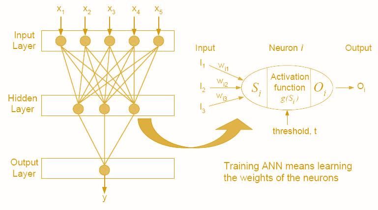
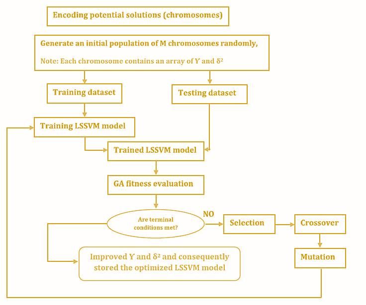
Preprints (www.preprints.org) | NOT PEER-REVIEWED | Posted: 6 February 2020 doi:10.20944/preprints202002.0075.v1

 7 of 30

 Fig. 2 The typical configuration of the LSSVM approach.

 In which P is the RH, subscripts rep/pred and exp denote the estimated and measured RH,
 correspondingly, and ns stands for the number of samples. The goal of this approach is to determine
 optimal dependent variables (i.e., σ2 and γ). In this regard, several optimization methods including
 Back Propagation (BP), Particle Swarm Optimization (PSO), Genetic Algorithm (GA), Hybrid Particle
 Swarm Optimization and Genetic Algorithm (HPSOGA), Imperialist Competitive Algorithm (ICA),
 and Unified Particle Swarm Optimization (UPSO) can be applied. In the present work, we used
 Genetic Algorithm to optimize σ2 and γ. The flow diagram of this approach is shown in Fig. 2.

 2.3 Artificial neural network (ANN)

 As observed in Fig. 3, the multilayer perceptron (MLP) neural network is created from input, hidden,
 and output layers. In this structure, the number of hidden layers may be one or more. Each layer
 consists of some neurons that their number should be specified by optimization techniques or trial
 and error procedures. In order to learn the ANN model, the parameters are adjusted till minimum
 square error (MSE) is obtained. In MLP structure of ANN usually, is optimized by back-propagation
 technique. The optimized number of iterations which is named by epochs must be used to determine
 the weights and biases to overcome undertraining and overtraining problems. These problems lead
 to obtaining poor results at testing phase [22,23].

Preprints (www.preprints.org) | NOT PEER-REVIEWED | Posted: 6 February 2020 doi:10.20944/preprints202002.0075.v1

 8 of 30

 Fig. 3 Structure of typical MLP artificial neural network.

 There is a distinct computation in the structure of the MLP and RBF, while their utilizations are
 similar. Owning to the simple design of the RBF frameworks (see Fig. 4), they have more advantages
 than MLP structure. This distinction makes the RBF structure more capable for generalization of
 outcomes [24].
 RBF framework is a kind of iterative function estimator which is used the concentrated basis functions.
 In order to create a model, this framework uses a supervisory training technique that is a kind of
 feed-forward neural network.

 Fig. 4 Scheme of typical RBF-ANN.

Preprints (www.preprints.org) | NOT PEER-REVIEWED | Posted: 6 February 2020 doi:10.20944/preprints202002.0075.v1

 9 of 30

 Thanks to RBF structure, its computations is much simpler and quicker than MLP structure. The RBF
 configuration is similar to the conventional regularization framework. Three advantageous features
 of regularization framework are expressed as follows:
 • Its capability to estimate any multivariate nonstop function on a compressed domain in order
 to a reach satisfactory outcomes through utilization of an adequate number of components.
 • The best solution is determined with minimization of a function that indicates its oscillation.
 • Owning to the linear configuration of unidentified coefficients, there is the best estimation
 feature.

 As shown in above two figures, the scheme of the RBF is nearly similar to the MLP. It has three layers;
 an output layer, an input layer, and a hidden layer. However, the main distinctions of these two
 configurations including:
 • RBF framework uses the easier construction than MLP.
 • There is much simpler training process in RBF framework than MLP.
 • MLP structure acts globally and its outcomes are specified through the relationship between
 all the neurons, while the RBF structure acts locally and its outcomes are determined by
 identified hidden units in particular local accessible areas.
 • The classification manners in these frameworks are different. Separation of each cluster is
 performed by the hypersurfaces in the MLP structure, while this task is done by the
 hyperspheres in RBF configuration.
 3. Development of Models

 The precise experimental relative humidity values are required to evolve aforementioned models. In
 this study, we used the relative humidity, wet bulb depression, and temperature that have been
 recorded in the reference and their ranges were presented in Table 1 [15].

 The next stage is the selection of inputs and target variables of models. To that end, the wet-bulb
 depression and temperature are given as inputs and relative humidity is regarded as the target
 parameter. The database used in this study consists of 330 data points. This data set should be divided
 into two datasets namely, training and testing sets, to train and test the capability of proposed models.

 Table 1 Ranges of data employed in the present study.

 Wet-bulb depression, Cº Dry bulb temperature, Cº Humidity

 -10 1-30 7-92

 -5 1-30 8-93

 0 1-30 8-93

 5 1-30 9-93

 10 1-30 10-94

 15 1-30 11-94

Preprints (www.preprints.org) | NOT PEER-REVIEWED | Posted: 6 February 2020 doi:10.20944/preprints202002.0075.v1

 10 of 30

 20 1-30 12-94

 25 1-30 13-94

 30 1-30 14-94

 35 1-30 16-95

 40 1-30 17-95

 The training data set contains 248 data points which are approximately 75% of total data points and
 the remained data points were used for testing. In addition, these data points were normalized within
 the ranges of -1 and +1 to achieve better performance with these models.

 As mentioned, in the current work, four models based on machine learning concepts including, the
 ANFIS, LSSVM, and two kind of ANN namely the MLP and RBF structures were evolved to predict
 the relative humidity using wet bulb depression and dry bulb temperature. There are two parameters
 in the LSSVM which require being adjusted before the training step. The regularization parameter (γ)
 and the kernel parameter corresponding to the kernel type (σ2) are the LSSVM tuned parameters.
 Moreover, the ANFIS method have some membership functions which have parameters. The optimal
 values of membership function parameters should be determined to reach the optimal ANFIS
 structure. The widely applied membership functions are the Generalized bell, Triangular, Gaussian,
 and Trapezoidal. In addition, the best number of hidden neurons in the structure of RBF and MLP
 artificial neural network should be used to obtain best values for weights and biases.

 Consequently, the performance analysis should be performed to evaluate model’s capability. In this
 regard, different statistical analyses such as the Average Absolute Error (AAE), Mean Squared Errors
 (MSEs), Mean Relative Errors (MREs), Root Mean Square Error (RMSE), Standard Deviations (STD),
 and the R-squared (R2) were performed between the real and predicted data by the models. These
 analyses can be expressed as follows:

 1
 ∑
 = ∑ =1( 2 (31)
 
 1 N  exp −  cal
 MRE =
 N
 
 i =1  exp
 (32)

 1
 ∑
 = ∑ =1| |||
 
 (33)

 1 0.5
 = ( ∑ 2
 =1( − ) ) (34)
 −1

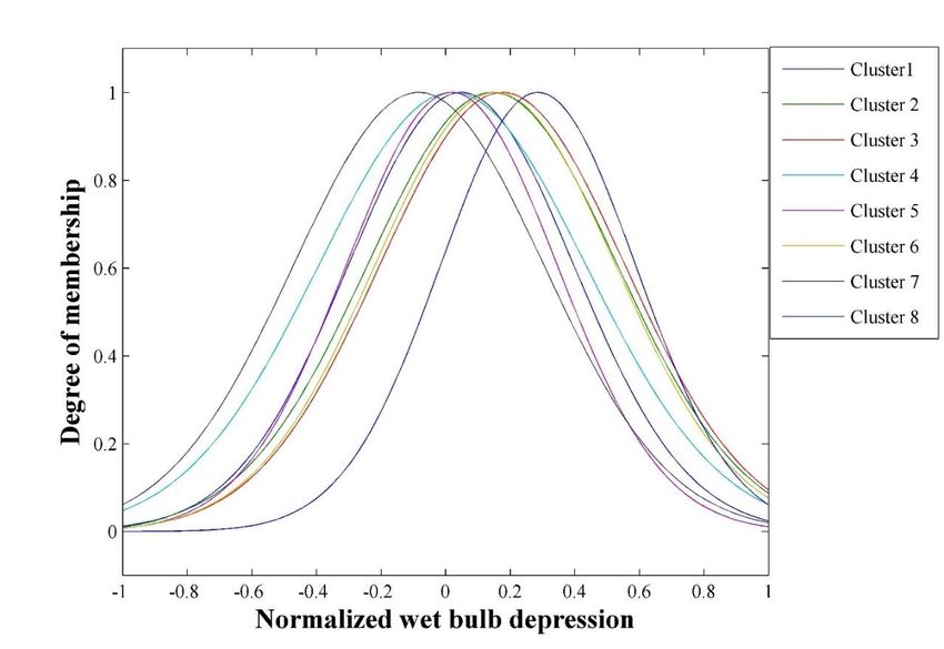
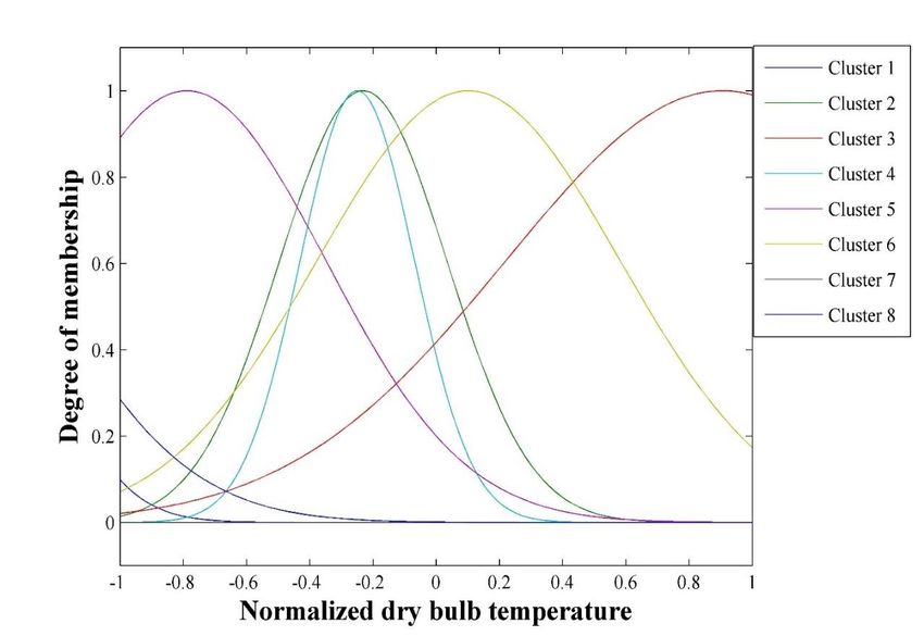
Preprints (www.preprints.org) | NOT PEER-REVIEWED | Posted: 6 February 2020 doi:10.20944/preprints202002.0075.v1

 11 of 30

 ∑ 1
 = ( ∑ =1( 2 ()0.5 ) (35)
 
 (36)

 Where αexp and αcal stand for the experimental and determined data point by algorithms respectively.
 In addition, N stands for the number of data points.

 4. Results and Discussions

 We used the RBF as kernel function of the LSSVM method. The RBF parameters have a significant
 effect on the number of support vectors. The more the number of support vectors, the more the
 elapsed training time. The optimal values of the LSSVM parameters namely, the kernel parameter
 (σ2) and the regularization parameter (γ) have been calculated using a genetic algorithm (GA). The
 GA is a straightforward strategy that uses concepts based on the natural selection for discovering the
 search space to reach a global optimum.

 Moreover, the membership function implemented in the ANFIS algorithm has chosen the Gaussian
 function due to its high efficiency in practice. We implemented a combination of genetic algorithm
 and ANFIS to reach the best structure. Moreover, this work used 8 clusters for the ANFIS and the
 total number of membership function parameters obtained 48. Going to the clarification, each
 Gaussian membership functions have two parameters and the number of input and output variables
 are two (wet bulb depression and dry bulb temperature) and one (relative humidity) respectively.
 Thus, based on the 8 clusters and three variables, the overall number of membership function
 parameters is determined as follows:

 Total Number of MF parameters = (Number of clusters) × (Number of variables) ×
 (number of MF parameter) (37)

Preprints (www.preprints.org) | NOT PEER-REVIEWED | Posted: 6 February 2020 doi:10.20944/preprints202002.0075.v1

 12 of 30

 Fig. 5 RMSE for combination of GA and ANFIS during different iterations.

 The performance of ANFIS based on RMSE of the determined and real values of humidity is
 shown in Fig. 5. As depicted, the maximum number of iterations was chosen 1000 and the optimum
 of RMSE was achieved as 0.40504. Fig. 6 illustrates trained membership function parameters for input
 variables including the wet bulb depression and dry bulb temperature, respectively. Their values
 vary between -1 and +1, because of normalizing.

 We used the linear transfer function and Log-Sigmoid transfer function in the output and
 hidden layers of suggested MLP-ANN model, respectively. In addition, we apply trial and error
 procedure to obtain an optimum number of neurons in its hidden layer. We used 7 neurons in the
 hidden layer and trained the MLP-ANN by the back-propagation technique. Table 2 presents
 obtained tuning parameters of weight and bias. Furthermore, as mentioned in theory section, the
 radial basis transfer functions (RBF) apply in the RBF-ANN model. The number of iterations is equal
 to the number of hidden neurons. Based on learning technique, the values of MSE was indicated in
 Fig. 7 for the duration of different iterations.

 (a)

Preprints (www.preprints.org) | NOT PEER-REVIEWED | Posted: 6 February 2020 doi:10.20944/preprints202002.0075.v1

 13 of 30

 (b)

 Fig. 6 The membership functions for (a) wet bulb depression and (b) dry bulb temperature.

 Details of suggested algorithms have been reported in Table 3.

 Table 2 Trained values of bias and weight for the MLP-ANN algorithm.

 Neuron Hidden layer Output layer

 Weight Bias Weight Bias

 Wet bulb Dry bulb B1 Humidity B2
 depression Temperature

 1 348.1958 168.1785 -75.9982 2.40597 -548.86

 2 -692.671 539.7101 85.76041 -0.76683

 3 -75.0567 -702.666 434.4219 -0.16664

 4 0.31539 -1.49156 -3.57515 1879.579

 5 -0.62346 2.066118 3.396896 550.1567

Preprints (www.preprints.org) | NOT PEER-REVIEWED | Posted: 6 February 2020 doi:10.20944/preprints202002.0075.v1

 14 of 30

 Fig. 7 Performance of RBF-ANN model at training stage.

 Table 3 Details of the suggested models for the determination of relative humidity.

 LSSVM ANFIS

Preprints (www.preprints.org) | NOT PEER-REVIEWED | Posted: 6 February 2020 doi:10.20944/preprints202002.0075.v1

 15 of 30

 MLP-ANN RBF-ANN

 The actual against estimated relative humidity by the models have been illustrated in terms of wet
 bulb depression and dry bulb temperature in Fig. 8. In addition, the actual and predicted relative
 humidities are indicated simultaneously in Fig. 9 at training and testing stages. All models predict
 the relative humidity nicely and a reasonable agreement with the real data represents their
 capabilities. In Table 4, a comparison was done between the developed model by Bahadori et al.
 and our suggested models in this study. According to obtained outputs from the models, all
 approaches have a very good agreement with actual reported data and this comparison indicates
 their satisfactory performance.

Preprints (www.preprints.org) | NOT PEER-REVIEWED | Posted: 6 February 2020 doi:10.20944/preprints202002.0075.v1

 16 of 30

Preprints (www.preprints.org) | NOT PEER-REVIEWED | Posted: 6 February 2020 doi:10.20944/preprints202002.0075.v1

 17 of 30

 Fig. 8 The performance of predictive methods in comparison with the actual data for determining
 relative humidity.

Preprints (www.preprints.org) | NOT PEER-REVIEWED | Posted: 6 February 2020 doi:10.20944/preprints202002.0075.v1

 18 of 30

Preprints (www.preprints.org) | NOT PEER-REVIEWED | Posted: 6 February 2020 doi:10.20944/preprints202002.0075.v1

 19 of 30

 Fig. 9 Actual versus estimated relative humidity by: (a) LSSVM, (b) ANFIS, (c) MLP-ANN, and (d)
 RBF-ANN.

Preprints (www.preprints.org) | NOT PEER-REVIEWED | Posted: 6 February 2020 doi:10.20944/preprints202002.0075.v1

 20 of 30

Preprints (www.preprints.org) | NOT PEER-REVIEWED | Posted: 6 February 2020 doi:10.20944/preprints202002.0075.v1

 21 of 30

 Fig. 10 Regression plots estimation of the relative humidity by: (a) LSSVM, (b) ANFIS, (c) MLP-
 ANN, and (d) RBF-ANN.

Preprints (www.preprints.org) | NOT PEER-REVIEWED | Posted: 6 February 2020 doi:10.20944/preprints202002.0075.v1

 22 of 30

 The regression analysis has been shown in Fig. 10 for all models at training and testing phases.
 According to statistical knowledge, the R2 value is a well-known term which indicates the
 relationship between the model outputs and real values. Whereas R2 = 1, an interesting linear
 relationship is established between the predicted and real values. Conversely, as R2 is closer to zero,
 the linear relationship between the predicted and real values is weaker. A close-fitting of data points
 around the 45° line for the predictive tools represent the precision.

 Table 4 Comparison of the suggested algorithms with Bahadori et al. approach [9]

 Temperature, Wet bulb Reported Bahadori LSSVM ANFIS RBF- MLP-
 Cº depression, RH% et al. ANN ANN
 Cº model

 -10 1 92 92.7 92.00 92.32 91.46 88.57

 0 2 86 86.4 86.18 86.44 86.06 85.57

 10 3 82 81.5 81.72 81.66 82.16 82.30

 20 4 78 77.6 77.82 77.65 77.76 78.06

 30 5 75 74.5 74.65 74.48 74.35 75.71

 40 6 72 72.1 72.04 72.05 72.04 70.43

 -10 7 57 56.3 56.75 56.83 56.58 56.87

 0 8 55 54.6 54.80 55.25 54.94 55.54

 10 9 54 53.4 53.44 53.53 53.42 54.69

 20 10 53 52.4 52.50 52.42 52.71 52.76

 30 11 52 51.7 51.82 51.87 52.03 52.91

 40 12 51 51.1 51.17 51.21 51.24 50.29

 -10 13 34 33.7 33.70 34.35 33.83 35.01

 0 14 34 33.9 34.00 34.38 34.15 34.61

 10 15 34 34.3 34.25 34.32 34.31 34.08

 20 16 35 34.8 34.72 34.69 34.67 35.04

 30 17 35 35.3 35.37 35.34 35.35 35.72

 40 18 36 35.7 35.92 35.89 35.89 34.68

 -10 19 20 19.6 19.66 20.73 19.19 20.85

Preprints (www.preprints.org) | NOT PEER-REVIEWED | Posted: 6 February 2020 doi:10.20944/preprints202002.0075.v1

 23 of 30

 0 20 21 20.5 20.56 21.02 19.02 19.06

 10 21 22 21.5 21.51 21.55 19.89 18.99

 20 22 23 22.6 22.56 22.48 20.82 21.26

 30 23 24 23.6 23.70 23.57 23.55 23.45

 40 24 25 24.6 24.70 24.74 24.81 23.29

 -10 25 11 11 11.19 11.56 11.13 12.17

 0 26 12 11.9 11.92 12.22 11.84 12.39

 10 27 13 13 13.08 13.17 13.13 12.41

 20 28 14 14.2 14.25 14.30 14.07 14.82

 30 29 15 15.4 15.32 15.47 15.24 14.79

 40 30 17 16.8 16.89 16.54 17.01 15.49

 The obtained linear regressions of the LSSVM, ANFIS, MLP-ANN, and RBF-ANN from the statistical
 analyses were expressed respectively as follows:

 y = 0.9963 x + 0.1817; R² = 0.9998 (38)

 y = 0.9993 x − 0.0099; R² = 0.9996 (39)

 y = 0.9963 x + 0.1817; R² = 0.9998 (40)

 y = 0.9993 x − 0.0099; R² = 0.9996 (41)

 Table 5 the statistical analyses of proposed models

 Model R2 MSE MRE (%) RMSE STD

 LSSVM Train 0.9999 0.062767 0.731401 0.250534 0.250534

 Test 0.999757 0.131755 0.931285 0.36298 0.36266

 ANFIS Train 0.999791 0.130927 1.198856 0.361839 0.361839

 Test 0.999627 0.193009 1.296151 0.439328 0.437627

 MLP-ANN Train 0.998747 0.784485 2.730389 0.885711 0.885711

 Test 0.998085 1.001084 2.388525 1.000542 0.995979

Preprints (www.preprints.org) | NOT PEER-REVIEWED | Posted: 6 February 2020 doi:10.20944/preprints202002.0075.v1

 24 of 30

 RBF-ANN Train 0.999912 0.055023 0.644804 0.23457 0.234569

 Test 0.999746 0.134121 0.933355 0.366225 0.363983

 Besides above illustrations, the capability of aforementioned models was evaluated using the MSE,
 MRE, STD, RMSE, and R2. These statistical parameters have been summarized in Table 5.
 Furthermore, the relative deviation percentages between the actual and estimated value of relative
 humidity by the models has been indicated in Fig. 11.

Preprints (www.preprints.org) | NOT PEER-REVIEWED | Posted: 6 February 2020 doi:10.20944/preprints202002.0075.v1

 25 of 30

 Fig. 11 The absolute relative deviation between the model outputs and actual values for: (a) LSSVM,
 (b) ANFIS, (c) MLP-ANN, and (d) RBF-ANN models.

Preprints (www.preprints.org) | NOT PEER-REVIEWED | Posted: 6 February 2020 doi:10.20944/preprints202002.0075.v1

 26 of 30

 (a)

 (b)

Preprints (www.preprints.org) | NOT PEER-REVIEWED | Posted: 6 February 2020 doi:10.20944/preprints202002.0075.v1

 27 of 30

 Fig. 12 William’s plots for (a) LSSVM, (b) ANFIS, (c) MLP-ANN, and (d) RBF-ANN models.

 In order to determine outliers of models, William's plot was utilized. This figure illustrates the
 standardized residuals versus hat values. Fig. 12 indicates the outlier analysis of the aforementioned
 models. Three limited boundaries can be obvious in these plots including leverage limit, upper and
 down suspected limit. Only the data with higher standardized residual values than 3 or lower than -

Preprints (www.preprints.org) | NOT PEER-REVIEWED | Posted: 6 February 2020 doi:10.20944/preprints202002.0075.v1

 28 of 30

 3 are outliers and the data with hat>hat* are out of applicability domain of the applied models. The
 term hat* refers to warning leverage value and for the present models, the warning value obtained
 0.027. More information can be found in the literature regarding William's plot [10,18,25].

 Consequently, the ability of these proposed tools was significantly confirmed by the great agreement
 between the estimated data and the real data in evaluating the models for the training and testing
 stages.

 5. Conclusion

 The aim of this study was to investigate the potential of four models based on statistical learning
 concepts, such as ANFIS, LSSVM, RBF, and MLP artificial neural network for predicting relative
 humidity by dry bulb temperature and wet bulb depression. The membership function parameters
 of the ANFIS and the LSSVM parameters (i.e. the regularization parameter and kernel parameter)
 were determined through the genetic algorithm. The genetic algorithm had good performance to
 adjust their tuning parameters. Estimations were indicated to be in a close match with actual data
 points. Based on the results obtained by statistical analyses, the ability of the proposed methods was
 significantly confirmed by the good agreement between the estimated data and the real data in
 evaluating the models for the training and testing stages. In addition, outcomes of suggested models
 have been compared with another reported correlation and the accuracy of models was proved as
 expected. Unlike complex mathematical approaches for prediction of relative humidity, the
 suggested approaches are user-friend and would be of excellent help for scientists especially in
 cooling towers and air conditioning systems.

 References

 1. Przybylak, R. Air Humidity. In The Climate of the Arctic; Springer, 2016; pp. 127–136.

 2. Vicente-Serrano, S.M.; Gimeno, L.; Nieto, R.O.; Azorin-Molina, C. Global Changes In Relative
 Humidity: Moisture Recycling, Transport Processes And Implications For Drought Severity.
 In Proceedings of the AGU Fall Meeting Abstracts; 2016.

 3. Hasan, A. Indirect evaporative cooling of air to a sub-wet bulb temperature. Appl. Therm. Eng.
 2010, 30, 2460–2468.

 4. Shallcross, D.C. Preparation of psychrometric charts for water vapour in Martian atmosphere.
 Int. J. Heat Mass Transf. 2005, 48, 1785–1796.

 5. Zhao, X.; Li, J.M.; Riffat, S.B. Numerical study of a novel counter-flow heat and mass
 exchanger for dew point evaporative cooling. Appl. Therm. Eng. 2008, 28, 1942–1951.

 6. Mohanraj, M.; Jayaraj, S.; Muraleedharan, C. Applications of artificial neural networks for
 refrigeration, air-conditioning and heat pump systems—A review. Renew. Sustain. Energy Rev.
 2012, 16, 1340–1358.

 7. Hasan, A. Going below the wet-bulb temperature by indirect evaporative cooling: analysis
 using a modified ε-NTU method. Appl. Energy 2012, 89, 237–245.

Preprints (www.preprints.org) | NOT PEER-REVIEWED | Posted: 6 February 2020 doi:10.20944/preprints202002.0075.v1

 29 of 30

 8. Singh, A.K.; Singh, H.; Singh, S.P.; Sawhney, R.L. Numerical calculation of psychrometric
 properties on a calculator. Build. Environ. 2002, 37, 415–419.

 9. Bahadori, A.; Zahedi, G.; Zendehboudi, S.; Hooman, K. Simple predictive tool to estimate
 relative humidity using wet bulb depression and dry bulb temperature. Appl. Therm. Eng. 2013,
 50, 511–515.

 10. Baghban, A.; Bahadori, A.; Mohammadi, A.H.; Behbahaninia, A. Prediction of CO2
 loading capacities of aqueous solutions of absorbents using different computational schemes.
 Int. J. Greenh. Gas Control 2017, 57.

 11. Baghban, A.; Bahadori, M.; Rozyn, J.; Lee, M.; Abbas, A.; Bahadori, A.; Rahimali, A. Estimation
 of air dew point temperature using computational intelligence schemes. Appl. Therm. Eng.
 2016, 93.

 12. Baghban, A.; Kardani, M.N.; Habibzadeh, S. Prediction viscosity of ionic liquids using a
 hybrid LSSVM and group contribution method. J. Mol. Liq. 2017, 236.

 13. Baghban, A.; Mohammadi, A.H.; Taleghani, M.S. Rigorous modeling of CO2
 equilibrium absorption in ionic liquids. Int. J. Greenh. Gas Control 2017, 58.

 14. Baghban, A.; Pourfayaz, F.; Ahmadi, M.H.; Kasaeian, A.; Pourkiaei, S.M.; Lorenzini, G.
 Connectionist intelligent model estimates of convective heat transfer coefficient of nanofluids
 in circular cross-sectional channels. J. Therm. Anal. Calorim. 2017.

 15. Burger, R.M. Engineering Design Handbook. Nat. Environ. Factors, Dep. Army, Richmond, VA
 1975.

 16. Jang, J.-S.R. Neuro-Fuzzy and Soft Computing/J.-SR Jang, C.-T. Sun, E. Mizutani. A Comput.
 Approach to Learn. Mach. Intell. Saddle River, NJ Prentice Hall, Inc., 1997.–614 p 1997.

 17. Jang, J.-S.R.; Sun, C.-T.; Mizutani, E. Neuro-fuzzy and soft computing; a computational
 approach to learning and machine intelligence. 1997.

 18. Baghban, A.; Sasanipour, J.; Haratipour, P.; Alizad, M.; Vafaee Ayouri, M. ANFIS modeling
 of rhamnolipid breakthrough curves on activated carbon. Chem. Eng. Res. Des. 2017, 126.

 19. Buragohain, M.; Mahanta, C. A novel approach for ANFIS modelling based on full factorial
 design. Appl. Soft Comput. 2008, 8, 609–625.

 20. Suykens, J.A.K.; Van Gestel, T.; De Brabanter, J. Least squares support vector machines; World
 Scientific, 2002; ISBN 9812381511.

 21. Ye, J.; Xiong, T. Svm versus least squares svm. In Proceedings of the International Conference
 on Artificial Intelligence and Statistics; 2007; pp. 644–651.

 22. Mitchell, T.M. Artificial neural networks. Mach. Learn. 1997, 45, 81–127.

 23. Dayhoff, J.E.; DeLeo, J.M. Artificial neural networks. Cancer 2001, 91, 1615–1635.

Preprints (www.preprints.org) | NOT PEER-REVIEWED | Posted: 6 February 2020 doi:10.20944/preprints202002.0075.v1

 30 of 30

 24. Park, J.; Sandberg, I.W. Approximation and radial-basis-function networks. Neural Comput.
 1993, 5, 305–316.

 25. Baghban, A.; Mohammadi, A.H.; Taleghani, M.S. Rigorous modeling of CO 2 equilibrium
 absorption in ionic liquids. Int. J. Greenh. Gas Control 2017, 58, 19–41.