On the information hidden in a classifier distribution - Nature
←
→
Page content transcription
If your browser does not render page correctly, please read the page content below
www.nature.com/scientificreports
OPEN On the information hidden
in a classifier distribution
Farrokh Habibzadeh1,4*, Parham Habibzadeh2,4, Mahboobeh Yadollahie1 &
Hooman Roozbehi3
Classification tasks are a common challenge to every field of science. To correctly interpret the
results provided by a classifier, we need to know the performance indices of the classifier including its
sensitivity, specificity, the most appropriate cut-off value (for continuous classifiers), etc. Typically,
several studies should be conducted to find all these indices. Herein, we show that they already exist,
hidden in the distribution of the variable used to classify, and can readily be harvested. An educated
guess about the distribution of the variable used to classify in each class would help us to decompose
the frequency distribution of the variable in population into its components—the probability density
function of the variable in each class. Based on the harvested parameters, we can then calculate
the performance indices of the classifier. As a case study, we applied the technique to the relative
frequency distribution of prostate-specific antigen, a biomarker commonly used in medicine for the
diagnosis of prostate cancer. We used nonlinear curve fitting to decompose the variable relative
frequency distribution into the probability density functions of the non-diseased and diseased people.
The functions were then used to determine the performance indices of the classifier. Sensitivity,
specificity, the most appropriate cut-off value, and likelihood ratios were calculated. The reference
range of the biomarker and the prevalence of prostate cancer for various age groups were also
calculated. The indices obtained were in good agreement with the values reported in previous studies.
All these were done without being aware of the real health status of the individuals studied. The
method is even applicable for conditions with no definite definitions (e.g., hypertension). We believe
the method has a wide range of applications in many scientific fields.
Classification tasks are a common challenge to every field of science. We often need to categorize a new observa-
tion into one of predefined groups based on its attributes. The definitions provided for a classifier varies a little
bit from field to field. In statistics, a classifier is an algorithm that help us with data c ategorization1. In machine
learning, the function of a classifier is to map objects based on their features to c lasses2. In medicine, a classi-
fier can be considered a diagnostic test helping physicians to classify people to healthy and diseased groups3.
Classifiers are extensively used in various disciplines of science. A classifier can be used for categorization of
an incoming e-mail into spam and non-spam, based on its contents4; stars into spectral types, based on their
diffraction pattern5; and tumors to benign or malignant, based on a b iomarker6, to name just a few applications.
There are several performance indices for the assessment of a classifier. The performance of a binary classifier
in classifying a binary attribute, typically involves comparing results of two methods—a gold-standard method
and the classifier being tested. In this way, we can determine the true-positive rate or sensitivity (Se), the true-
negative rate or specificity (Sp), and the likelihood ratio of a positive or negative results for the classifier7. Typi-
cally, several studies should be conducted to find these values. Herein, we show that all these indices are already
available, hidden in the distribution of the variable used to classify and can readily be harvested. We present a
method to harvest the indices. An educated guess about the distribution of the variable used to classify in each
class would help us to decompose the frequency distribution of the variable in population into its components—
the probability density function of the variable in each class. Based on the harvested parameters, we can then
calculate the performance indices of the classifier. As an example for the application of the proposed method, we
use the frequency distribution of prostate-specific antigen (PSA), an immunologic biomarker commonly used
for the diagnosis of prostate cancer, and compare the results to values reported in previous studies.
1
R&D Headquarters, Petroleum Industry Health Organization Polyclinic, Eram Blvd, 7143837877 Shiraz,
Iran. 2Persian BayanGene Research and Training Center, Shiraz University of Medical Sciences, Shiraz,
Iran. 3Peyvand Clinical Laboratory, Shiraz, Iran. 4These authors contributed equally: Farrokh Habibzadeh and
Parham Habibzadeh. *email: Farrokh.Habibzadeh@gmail.com
Scientific Reports | (2021) 11:917 | https://doi.org/10.1038/s41598-020-79548-9 1
Vol.:(0123456789)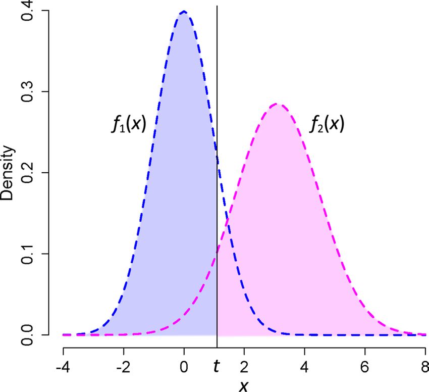
www.nature.com/scientificreports/
Case study. PSA is commonly used for the diagnosis of prostate cancer. In this case study, we use PSA values
for the categorization of patients into two groups of “non-diseased” and “diseased.” However, to correctly inter-
pret the PSA results, we need to know the reference range of the test value; the most appropriate cut-off value for
PSA above which the test is considered positive3; what percentage of a population has the disease (prevalence
or the prior probability of the disease [pr]); the probability that the test becomes positive in a diseased person
(true-positive rate or test sensitivity [Se]); the probability that a non-diseased person becomes test-negative
(true-negative rate or test specificity [Sp]); the false-positive and false-negative rates and an estimation of their
costs; the likelihood ratio of a positive or negative test result or the likelihood ratio for a certain PSA v alue6,8, etc.
Several studies have so far been conducted to find all these indices. Herein, we harvest these values from the fre-
quency distribution of PSA measured in a group of people. Nonetheless, the very first step is taking an educated
guess about the distribution of PSA in non-diseased and diseased people.
Hypothesis about the distribution of PSA. The distribution of PSA in healthy people and those with prostate
cancer is positively skewed. However, with acceptable clinical accuracy, after a logarithmic transformation, it
has a normal distribution in both non-diseased and diseased people; Ln(PSA) has a binormal distribution in the
population (consisting of both non-diseased and diseased individuals)9.
The general form of a normal distribution with a mean of µ and the standard deviation (SD) of σ is3:
1 −(x−µ)2
f x|µ, σ 2 = √
e 2σ 2
2π σ
(1)
1 x−µ
= ϕ
σ σ
where φ represents the probability density function of the distribution. A binormal distribution, the superposi-
tion of two normal distributions, thus, has the following general equation:
a 1 − pr
x − µ1 a pr x − µ2
y(x) = ϕ + ϕ (2)
σ1 σ1 σ2 σ2
where, μ1, σ1, μ2, and σ2 represent mean and the SD of Ln(PSA) in the non-diseased and diseased people, respec-
tively; pr represents the prior probability (prevalence, if no other information is available) of the disease; and a
is a correction factor.
Equation 2 is a little bit different from the three-parameter binormal equation commonly mentioned in the
literature10. The three-parameter distribution, in fact, includes two half-Gaussian distributions. Each point of the
distribution in Eq. 2 is the summation of two Gaussian distributions. Choosing Eq. 2 for our model was rooted
in our hypothesis that normal prostate cells are a homogenous population of cells producing PSA, the amount of
which increases by age11. Prostate malignant cells, on the other hand, are heterogenous in genotype and produce
a wide range of PSA, the amount of which is not age-dependent12,13. We therefore assumed two independent
populations of cells—a population of homogenous normal prostate cells producing PSA (the first term in Eq. 2)
with an age-dependent distribution, and a population of heterogenous prostate malignant cells producing PSA
(the second term in Eq. 2) the distribution of which is not age-dependent.
Frequency distribution of PSA. A large set of data, consisting of 18,561 records of PSA values taken from the
database of a general clinical laboratory in Shiraz, southern Iran, were used for analysis. PSA values were meas-
ured between March 2017 and September 2019. The values were then log-transformed. A histogram of the rela-
tive frequency distribution of Ln(PSA), was then constructed.
Results
An educated guess would help us to decompose the frequency distribution of the variable used to classify in
the population to its components—the probability distribution function of the variable in each group. Using a
nonlinear curve fitting, a binormal curve (our hypothesized distribution) was fitted to the relative frequency
distribution of Ln(PSA); the parameters of the probability density functions of the variable for non-diseased
and diseased groups were derived. Based on the harvested parameters, the classifier performance indices were
then calculated.
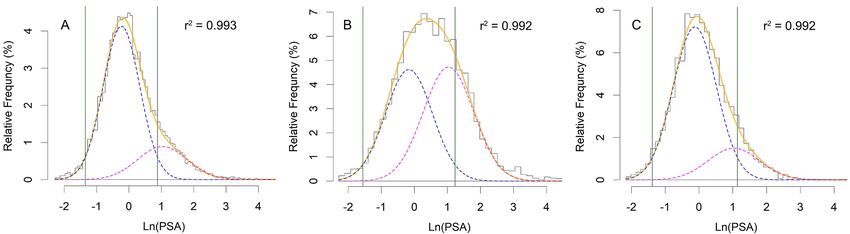
Frequency distribution of PSA. The relative frequency of Ln(PSA), as expected, had a good (r2 = 0.993)
fit to the hypothsized binormal distribution (Fig. 1A). Analysis of the subset data revealed that the distribution
of those aged ≥ 65 years (n = 4024) also had a good fit ( r2 = 0.992, Fig. 1B). In this subset, the maximum value for
the distribution of the diseased people (Fig. 1B, magenta dashed curve) was almost equal to that of non-diseased
people (blue dashed curve), indicating that the prevalence of the disease, pr in Eq. 2, is around 50%. Having a
similar weight, under this situation, μ2 and σ2 would be calculated with the same accuracy as μ1 and σ1 are.
Considering our hypothesis that there are two cell populations (non-diseased and diseased), and that the
distribution of PSA in the diseased group is not age-dependent, we used the estimations for μ2 and σ2 (the mean
and SD of Ln(PSA) for diseased population) that came from this age group for all other analyses. Assuming these
values, the relative frequency distribution of Ln(PSA) for those aged 54–59 years (n = 2781) had also a good fit
(r2 = 0.992, Fig. 1C). In fact, this assumption resulted in an acceptable fit ( r2 > 0.965) of a binormal distribution
(Eq. 2) to the observed distribution of data for all age groups studied.
Scientific Reports | (2021) 11:917 | https://doi.org/10.1038/s41598-020-79548-9 2
Vol:.(1234567890)www.nature.com/scientificreports/
Figure 1. Histograms of the relative frequency distribution of Ln(PSA) for (A) those aged ≥ 20 years, (B) ≥ 65,
and (C) 54–59 years. In each panel, the orange solid curve is the binormal curve fitted to the data (the histogram
representing the relative frequency). The curve is in fact the result of superposition of two normal curves
describing the relative frequency distribution of Ln(PSA) in non-diseased individuals (blue dashed curve) and
diseased patients (magenta dashed curve). Vertical green solid lines bound the reference range for PSA.
Figure 2. The reference range of the disease for each age. The values were obtained from subset analysis of data
of men aged 20–39, 40–49, 50–59, 60–69, 70–79, and ≥ 80 years. The two solid lines represent the lower and
upper limits of the reference range; dashed line, the 95th percentile of PSA. The values for each age group were
calculated based on the mean and SD of the distribution of Ln(PSA) in non-diseased people in each s ubset9.
Reference range of PSA. The reference range for a diagnostic test, here PSA, is important for clinicians.
The range is commonly defined as the interval between the 2.5th and 97.5th percentiles of the test value dis-
tribution in an apparently healthy p opulation14. Presuming a normal distribution for Ln(PSA) in non-diseased
individuals and given the mean and SD of the distribution (μ1 and σ1 for the dashed blue curves in Fig. 1) for each
age group, we calculated the reference range (μ1 ± 1.96 σ1) for Ln(PSA) (Fig. 1, the region bounded by vertical
green solid lines), and thus for PSA, as well as the 95th percentile of PSA for each age group (Fig. 2). The width
of the interval increased with age. This was mainly attributed to the increasing upper limit of the reference range
with age, an observation in concordance with what has been reported earlier in several studies conducted on
large number of people of various ethnic backgrounds15–20.
Prevalence of the disease. The prevalence of the disease for each age group was easily derived from the
curve fitting procedure. For example, the prevalence of the disease for 54–59-year-old men (n = 2781) was 19.8%.
There was a sharp increase in the prevalence between the age of 45 and 75 years (Fig. 3). It decreased thereafter.
Our results were in line with the reported results in the literature. Even, the observation that the prevalence
decreased slightly after the age of 75 was in line with the reported decrease in the incidence of the prostate cancer
after this age21,22.
There is a significant variation in the reported prevalence of prostate cancer among different populations. A
systematic review of published autopsy studies shows that the prevalence varies nonlinearly from 5% in those
aged < 30 years to 59% in men aged > 79 years23. Another forensic autopsy study conducted in Japan shows that
the prevalence increases by age—10.9% in 50’s, 17.1% in 60’s, and 21.2% in 70’s24. The corresponding values we
calculated were 16.5%, 40.6%, and 54.5%, respectively (Fig. 3). The observed difference mainly originated from
Scientific Reports | (2021) 11:917 | https://doi.org/10.1038/s41598-020-79548-9 3
Vol.:(0123456789)www.nature.com/scientificreports/
Figure 3. The prevalence of the disease for each age. The values were obtained from subset analysis of data
of men aged 20–39, 40–49, 50–59, 60–69, 70–79, and ≥ 80 years. The prevalence came directly from the curve
fitting.
our definition of the disease. While autopsy studies use various techniques (histopathology, histochemical stain-
ing, etc.) to identify malignant cells in tissue specimens, our method defines the disease based on the distribution
of PSA the prostate cells produce.
Tumors are generally not clinically detectable until they become as large as 1 cm in diameter (≈ 109 cells)12.
This represents around 75% of the natural history of the tumor; we can only diagnose a fraction of the tumors;
and that is why the prevalence of tumors in autopsy studies is much higher than that reported in clinical settings.
Nevertheless, there are tumors that are too small to be even identified in autopsy, whereas our method, which
is based on the distribution of PSA, can theoretically predict their presence; our method is even more sensi-
tive than the current autopsy techniques and that is why the prevalence we found was higher than the reported
figures in autopsy studies. The difference was higher for older men because the chance of developing malignant
cells significantly increased with age22.
Prostate cancer is typically a slow progressive disease. It has a long latent phase and many men with prostate
cancer die from other causes before their cancer being diagnosed at a ll24. This is why the reported prevalence
in live people diagnosed in a clinical setting is much lower than those reported in autopsy studies. For example,
in a study conducted in Japan, 170 of almost 24,000 men in their 60’s screened for prostate cancer, were found
positive, which translates to a prevalence of only 0.7%11. The study reports a prevalence of 0.3% in those aged
54–59; we came to a value of 19.8%. The tumor size in many of these people is too small to cause any problems
during the rest of their lives. These small tumors cannot be identified using the currently available diagnostic
modalities. The observed difference might also arise from the difference in the distribution of PSA among races19.
Based on our model, 67.8% of diseased people and 82% of 62–91-year-old men had a PSA ≤ 4 ng/mL. The
prevalence of the disease among this age group was 49.4%. Based on Bayes’ t heorem8,25, the probability that a
man aged 62–91 years with a PSA ≤ 4 ng/mL had cancer was 40.8%:
P(PSA ≤ 4|D+ )
P(D+ |PSA ≤ 4) = P(D+ )
P(PSA ≤ 4)
0.678
= × 0.494 = 0.408
0.820
where D+ represents presence of disease, and P(A | B) is the conditional probability of event A happens given the
event B has happened25. Considering the limitation of our current diagnostic tools mentioned above, this value
is in good agreement with the previous reported figure of 0.152 in the United States26.
Calculation of the sensitivity, specificity, the receiver operating characteristic (ROC) curve,
and the cut‑off value. Given the means and SDs of Ln(PSA) in diseased and non-diseased people and
considering normal distribution for both diseased and non-diseased people (based on our hypothesis), using
Eq. 12, we calculated the Se and Sp of the test assuming a cut-off value of t for Ln(PSA) as follows3:
+∞
1 x − µ2
Se(t) = ϕ dx
σ2 σ2
t
(3)
t − µ2
=1−�
σ2
Scientific Reports | (2021) 11:917 | https://doi.org/10.1038/s41598-020-79548-9 4
Vol:.(1234567890)www.nature.com/scientificreports/
Figure 4. ROC curve for 54–59-year-old men. The curve is constructed based on subset analysis of 54–59-year-
old men. The area under the curve is 0.874. The orange solid circle corresponds to the most appropriate cut-off
value for PSA, 1.61 ng/mL, a point maximizing the Youden’s index (corresponding to a relative cost of a false-
negative to a false-positive test result of 4), corresponding to a Se and Sp of 76.6% and 82.5%, respectively.
and
t
1 x − µ1
Sp(t) = ϕ dx
σ1 σ1
−∞ (4)
t − µ1
=�
σ1
where Φ represents the cumulative distribution function of the standard normal distribution. These calculations
were done for each age group. For example, for 54–59-year age group, μ1, σ1, μ2, and σ2 were -0.124, 0.643, 1.033,
and 0.766, respectively. Using Eqs. 3 and 4, the Se and Sp for a series of Ln(PSA) cut-off values were calculated,
based on which an ROC curve was constructed (Fig. 4)27,28. The area under the ROC curve was 0.874.
Based on the prevalence (19.8% for 54–59-year-old men in our example), and the cost of a false-negative
relative to a false-positive test result (arbitrarily chosen to be 4 in our example), the most appropriate test cut-
off value was calculated to be 1.61 ng/mL (the orange solid circle, Fig. 4). It corresponds to a Se and Sp of 76.6%
and 82.5%, r espectively3. This cut-off value also maximized the Youden’s index (Se + Sp − 1), an index reflecting
maximum potential effectiveness of a b iomarker3,29.
The most appropriate test cut-off value could be calculated for each age group. However, the cost of a false-
negative test result relative to a false-positive test result needs to be considered separately for different age groups.
For example, one may estimate it at 4 for 54–59-year-old men, and 0.2 for those aged 80 or more, as early diag-
nosis of the disease is not always good; it would increase the likelihood of harm rather than benefit because of
detection of clinically insignificant diseases, particularly at old ages30. Furthermore, the clinical relevance of the
inconclusive results obtained should be considered. There are various ways to handle the inconclusive results.
Two graphs ROCs is the easiest strategy to be u sed31; other techniques are more complex involving mathemati-
cal rigors32,33.
A study conducted in Japan proposed a cut-off value of 2.3 ng/mL for PSA in those aged 54–59 years11. This
value is less than the cut-off value of 3.0 set by the Japanese Urological Association for the age group. The cut-off
value of 2.3 ng/mL is associated with a test Se of 100% and a Sp of 92.3%11. Based on our results, however, the most
appropriate cut-off value was 1.61 ng/mL, which was associated with a Se and Sp of 76.6% and 82.5%, respectively.
The observed difference originated again from our case definition. While our model considers those with just a
few malignant cells “diseased,” the aforementioned study failed to diagnose the disease in them and thus falsely
categorized them into “non-diseased” group. This is also why in our model we set the cut-off to a lower value,
which decreases the test Sp. If we would have set our cut-off to 2.3 ng/mL (and missed many diseased people),
the Sp became 90.3%, very well comparable with that reported in the study11.
While some conditions, like prostate cancer, do have well-defined clinicopathological definitions, certain
disease conditions do not. For example, hypertension does not have such a well-defined clinicopathological defi-
nition. What we know for sure is that a higher blood pressure is associated with higher mortality and morbidity.
Nonetheless, we cannot define hypertension or give a certain cut-off value for classifying people according to
their blood pressure and assess the risk they bear. The cut-off values proposed for the diagnosis of hypertension
are constantly changing over time34. Our proposed method can probably identify the group of hypertensive and
Scientific Reports | (2021) 11:917 | https://doi.org/10.1038/s41598-020-79548-9 5
Vol.:(0123456789)www.nature.com/scientificreports/
Figure 5. Likelihood ratio (LR) for various PSA values in 54–59-year-old men. Note that both axes are
logarithms of the variables. The horizontal gray dashed line corresponds to an LR of 1; the vertical gray dashed
line represents the cut-off value, PSA of 1.61 ng/mL.
non-hypertensive people, and provide the reference range for blood pressure and the prevalence of hypertension
for each age group. In this way, we can have, once and for all, an invariant definition for hypertension.
Positive and negative predictive values. For a given cut-off value of t, and the prevalence of the disease,
we calculated the positive (PPV) and negative predictive values (NPV) using the following equations:
pr Se(t)
PPV (t) =
pr Se(t) + 1 − pr 1 − Sp(t)
(5)
1 − pr Sp(t)
NPV (t) =
1 − pr Sp(t) + pr(1 − Se(t))
Given the Se, Sp, pr of the disease, and the cut-off value of 1.61 ng/mL for PSA calculated for those aged
54–59 years, the PPV and NPV were 51.9% and 93.5%, respectively (Eq. 5).
Likelihood ratios. Positive and negative likelihood ratios (LR+ and LR–, respectively) for a given cut-off
value of t, were calculated as follows8:
Se(t)
LR+ (t) =
1 − Sp(t)
(6)
1 − Se(t)
LR− (t) =
Sp(t)
LR+ and LR– for the cut-off value of 1.61 ng/mL were 4.38 and 0.28, respectively (Eq. 6).
Having Se and Sp for two PSA values, it is possible to calculate the likelihood ratio for a range of P
SA8. For
example, based on the information obtained, the Se and Sp for a cut-off value for Ln(PSA) of 1.79 (PSA of 6 ng/
mL) were 16.1% and 99.9%, respectively; they were 32.2% and 99.1%, respectively, for a cut-off value for Ln(PSA)
of 1.39 (PSA of 4 ng/mL). The likelihood ratio for having a PSA between 4 and 6 ng/mL is t hus8:
Se(t1 ) − Se(t2 )
LR(t1 ≤ PSA < t2 ) = − (7)
Sp(t1 ) − Sp(t2 )
Therefore,
0.161 − 0.322
LR(4 ≤ PSA < 6) = − = 20
0.999 − 0.991
meaning that the probability of observing a PSA level between 4 and 6 ng/mL is 20 times more often in
54–59-year-old men with the disease compared with those without the d isease8.
Furthermore, because we derived the probability density function for the non-diseased and diseased groups,
we could calculate the likelihood ratio (LR) for any given PSA values in the studied group (e.g., 54–59-year-old
men) using the specific form of Eq. 13 (Fig. 5)8:
Scientific Reports | (2021) 11:917 | https://doi.org/10.1038/s41598-020-79548-9 6
Vol:.(1234567890)www.nature.com/scientificreports/
x−µ2
σ1 ϕ σ2
LR(x) =
x−µ1
(8)
σ2 ϕ σ1
where x is Ln(PSA). This is technically the slope of the line tangent to the ROC curve at the point corresponding
to the PSA value. In practice, it is very difficult to calculate this slope accurately, as the ROC curve is in fact just
a set of discrete points, not a differentiable curve8. Our method, however, can readily provide the information.
For example, the LR for Ln(PSA) of 1.79 (PSA of 6 ng/mL) was 43, meaning that in the age group of
54–59 years, a PSA level of 6 ng/mL was 43 times more likely to be observed in those with the disease as com-
pared with those without the disease8. On the other hand, the LR for Ln(PSA) of 0 (PSA of 1 ng/mL) was 0.34;
the likelihood of observing a PSA of 1 ng/mL in diseased people was one-third of those without the disease.
Conclusion
We showed that if we have an educated guess about the distribution of the variable used to classify, we can har-
vest the reference range for the variable; the prior probability of the condition of interest (here, prevalence of a
disease); the classifier performance indices including its Se, Sp, PPV, NPV, LRs, also the ROC curve and the area
under the curve, and the most appropriate cut-off value. However, to be sure about the frequency distribution of
the variable we need to perform an extensive sampling over all possible range of its values. Particular attention
should be paid to the extremes (tails) that might differentiate between the two classes, healthy and non-healthy
individuals.
In our case study, we assumed a binormal distribution for Ln(PSA) for a well-defined dichotomous condition,
diseased and non-diseased people. The method can be applied as well to those conditions without a well-defined
clinicopathological definition, say hypertension, and to other scientific disciplines.
The results calculated in our case study were based on the relative frequency distribution of the PSA and
an educated guess about the distribution of PSA in non-diseased and diseased people. No information about
the prostate cancer status of each individual studied was available. Our assumption to take the mean and SD of
Ln(PSA) of patients aged ≥ 65 years as an acceptable estimate for μ2 and σ2 for all other analyses, would seem
unacceptable at first glance, as those aged ≥ 65 made 22% of the total population studied. But, when we take
into account that more than half of all prostate cancers reported happen in this age group, the assumption made
might look reasonable. Furthermore, we hypothesized that the PSA distribution in diseased people is not age-
dependent. As a matter of fact, the essence of the work here is neither choosing the binormal distribution we
used for curve fitting nor our choice for μ2 and σ2; it is the way we could derive the test indices (Se, Sp, LRs, etc.)
solely based on an educated guess about the distribution of the variable used to classify, no matter how we become
aware of the distribution. In many instances, such as for the PSA9,31,33, there are enough evidence to help us with
making an educated guess and choosing a few appropriate distributions. Note that, if we had the distributions
of the variable for the groups, even in numeric forms, we could have calculated all the aforementioned indices
with numerical methods. Knowledge about the distribution of the variable in the classes help us with correct
decomposition of the population (non-diseased and diseased) relative frequency distribution (the histogram in
Fig. 1) into its components—the relative frequency distribution (and thus the probability density functions) of
the variable used to classify in each group (the blue and magenta dashed lines in Fig. 1).
The very good agreement between the results obtained from this method with those obtained independently
from prior research studies as well as the field-independency of the method proposed may in some way imply the
deep-seated mathematical rules in action in the nature from the microcosm within us and our surrounding world
to the macrocosm, the universe. We believe the method has a wide range of applications in many scientific fields.
Methods
Suppose a continuous classifier with a binary outcome. Let x be a random variable used to classify with prob-
ability density functions of fi(x) for the ith class. Let the classes be designated “negative” and “positive.” Assume
the lower values of the classifier belong to the negative class; the higher, to the positive. Comparing the results of
the classification against a gold-standard method gives four outcomes—true-positive (TP), false-positive (FP),
true-negative (TN), and false-negative (FN).
Prior probabilities. Assume that x is the variable used for the classification, and that pri designates the
probability that a randomly selected value of x being classified to class i—the prior probability. Then, the fre-
quency distribution for the variable x observed in the population, regardless of classes, should follow the general
equation:
n
F(x) = A pri fi (x) (9)
i=1
where A is a constant and 0 ≤ pri ≤ 1 for all i’s, and
n
pri = 1 (10)
i=1
An educated guess about the general form of the distribution of the variable used to classify in each class would
help us to decompose the frequency distribution of the variable in population, F(x), into its components—the
Scientific Reports | (2021) 11:917 | https://doi.org/10.1038/s41598-020-79548-9 7
Vol.:(0123456789)www.nature.com/scientificreports/
Figure 6. An example of the probability density functions of a continuous variable x used to classify the input
value to binary outcome (say a diagnostic test) for the negative class (f1(x), blue dashed line) and positive class
(f2(x), magenta dashed line). The negative and positive classes may correspond to non-diseased and diseased
people, respectively. The cut-off value of t is represented by the vertical solid line. The area under f2(x) to the
right of the cut-off value (the pink region) is then the sensitivity (Se), and the area under f1(x) to the left of the
cut-off value (the light blue region) is the specificity (Sp).
probability density function of the variable in each class, fi(x). We may estimate the pri and the parameters of the
distributions with nonlinear curve fitting procedures. Based on the harvested parameters, we can then calculate
the performance indices of the classifier.
Performance indices of the classifier. For a binary classifier (Fig. 6), the sensitivity (Se) and specificity
(Sp) of the classifier are defined as:
TP
Se =
TP + FN
(11)
TN
Sp =
TN + FP
The Se and Sp are functions of the classifier used. As an example, for our binary classifier (Fig. 6), for a cut-off
value of t, the functions are3:
+∞
Se(t) = f2 (x) dx
t
(12)
t
Sp(t) = f1 (x) dx
−∞
The receiver operating characteristic curve and the cut‑off value. Having Se and Sp corresponding
to various values of the variable used to classify, we can draw the receiver operating characteristic (ROC) curve
of the classifier and determine its most appropriate cut-off value3.
Likelihood ratio. For a binary classifier, the positive and negative likelihood ratio (LR+ and LR–, respec-
tively) associated with a cut-off value of t; the likelihood ratio for an interval [t1, t2), LR(t1 ≤ x < t2); and the likeli-
hood ratio for a certain value x, LR(x); can be derived as follows8:
Scientific Reports | (2021) 11:917 | https://doi.org/10.1038/s41598-020-79548-9 8
Vol:.(1234567890)www.nature.com/scientificreports/
Se(t)
LR+ (t) =
1 − Sp(t)
1 − Se(t)
LR− (t) =
Sp(t)
(13)
Se(t1 ) − Se(t2 )
LR(t1 ≤ x < t2 ) = −
Sp(t1 ) − Sp(t2 )
f2 (x)
LR(x) =
f1 (x)
Case study. Source of data. We analyzed the PSA values taken from the database of a general clinical labo-
ratory in Shiraz, southern Iran. Each day, the laboratory performs between 6000 and 8000 tests on samples re-
ceived from 600 to 800 people with various health states coming from various parts of Fars province. The values
were measured in samples received between March 2017 and September 2019 using electrochemiluminescence
immunoassay. To eliminate outliers, we only included the samples of men aged 20 years or above having PSA
values between 0.1 and 100 ng/mL.
Data analysis. Data analysis was performed with R software ver 4.0.2 (2020-06-22).
Construction of the histogram. To construct the histogram of the distribution of Ln(PSA), we first determined
the optimal size of the number of bins for each subset of the data. To determine the width of each bin, h, we used
Freedman-Diaconis rule as follows35:
2 IQR(x)
h= √3 (14)
n
where n is the sample size, x is Ln(PSA), and IQR(x) is the interquartile range of x. The optimal number of bins,
nbin, was then calculated as follows:
max(x) − min(x)
nbin = (15)
h
The relative frequency of Ln(PSA) for each bin was then calculated.
Decomposition of the frequency curve into its components. A nonlinear curve fitting function
(nlsLM() from minpack.ml package for R) was used to figure out the optimal values of parameters of a binormal
equation (Eq. 2) best fit to the frequency distribution (based on our hypothesis about the distribution of Ln(PSA)
in non-diseased and diseased people)36. The function works based on the Levenberg–Marquardt nonlinear least-
squares algorithm37. Constraints were imposed on the parameters a, σ1, and σ2 in Eq. 2—they could only assume
non-negative values; pr, the prior probability (prevalence) of the disease, could only assume values in the close
interval of [0, 1].
The pr for the disease for men aged ≥ 65 years was around 0.5. Under this circumstance, the two Gaussian-
distributed components (the two terms in Eq. 2) have an almost equal contribution to shaping the total distribu-
tion of PSA (Fig. 1); thus, μ2 and σ2 would be calculated with the same accuracy as μ1 and σ1 are. As we hypoth-
esized that the distribution of PSA in those with the disease is not age-dependent, we used the mean and SD of
Ln(PSA) obtained for men aged ≥ 65 with the disease (μ2 and σ2) as an estimate for the distribution of diseased
people for all other age groups studied. Therefore, in the first pass, we used a six-parameter binormal equation
(Eq. 2) for curve fitting for the age group of ≥ 65 to find the best estimates for μ2 and σ2; then, we assumed these
values fixed in the curve fitting looking for other parameters a, pr, μ1, and σ1, hence, a four-parameter model.
The reference range. In medical sciences, the reference range for diagnostic test results, here PSA, is important
and commonly defined as the interval between the 2.5th and 97.5th percentiles of the test value distribution in
an apparently healthy population14. Presuming a normal distribution for Ln(PSA) in non-diseased individuals
and given the mean and SD of the distribution (μ1 and σ1) for each age group, the reference range was calculated
as μ1 ± 1.96 σ1.
Prevalence of the disease. The prevalence of the disease for each age group was directly derived from the curve
fitting procedure, the pr in Eq. 2.
Calculation of the sensitivity and specificity. Given the means and SDs of Ln(PSA) in diseased and non-dis-
eased people and considering normal distribution for both diseased and non-diseased people (according to our
hypothesis), we simply calculated the Se and Sp of a test assuming a cut-off value of t for Ln(PSA) using Eqs. 3
and 4, respectively3. Considering the normal distribution of the classifier in our case study, Ln(PSA), in both
diseased and non-diseased people, given the cut-off value of t, we calculated the Se and Sp using the R function
pnorm() as follows:
Scientific Reports | (2021) 11:917 | https://doi.org/10.1038/s41598-020-79548-9 9
Vol.:(0123456789)www.nature.com/scientificreports/
Se < − pnorm(t, mean = µ2, sd = σ2, lower.tail = FALSE)
Sp < − pnorm(t, mean = µ1, sd = σ1, lower.tail = TRUE)
The receiver operating characteristic curve and the cut‑off value. The Se and Sp for a series of Ln(PSA) cut-off
values were calculated, based on which a receiver operating characteristic (ROC) curve was constructed. Then,
we calculated the most appropriate cut-off value for PSA3.
Positive and negative predictive values. Given the Se, Sp, and pr, we calculated the positive (PPV) and negative
predictive values (NPV) using Eq. 5.
Calculation of the likelihood ratios. Given the Se and Sp, various types of likelihood ratios were calculated using
Eqs. 6 to 88. Considering the binormal distribution of Ln(PSA) in diseased and non-diseased men, we calculated
the LR of x (Eq. 8), using the R function dnorm() that returns the density function of a normal distribution, as
follows8:
LRx < − dnorm(x, mean = µ2, sd = σ2)/dnorm(x, mean = µ1, sd = σ1)
Ethics. The study was conducted in accordance with the Declaration of Helsinki Code of Ethics. The study
protocol was approved by the Petroleum Industry Health Organization Institutional Review Board. Informed
consents were obtained from all participants. The authors did not have access to identifiable data records.
Data availability
The raw data and codes written in R are available from the journal Web site.
Received: 1 June 2020; Accepted: 10 December 2020
References
1. Sarma, K. V. S. & Vardhan, R. V. Multivariate Statistics Made Simple: A Practical Approach (CRC Press, Boca Raton, 2018).
2. Kotsiantis, S. Supervised machine learning: a review of classification techniques. Informatica (Ljubljana) 31, 249–268 (2007).
3. Habibzadeh, F., Habibzadeh, P. & Yadollahie, M. On determining the most appropriate test cut-off value: the case of tests with
continuous results. Biochem. Med. (Zagreb) 26, 297–307. https://doi.org/10.11613/BM.2016.034 (2016).
4. Dada, E. G. et al. Machine learning for email spam filtering: review, approaches and open research problems. Heliyon 5, e01802.
https://doi.org/10.1016/j.heliyon.2019.e01802 (2019).
5. Kuntzer, T., Tewes, M. & Courbin, F. Stellar classification from single-band imaging using machine learning. Astron. Astrophys.
591, A54. https://doi.org/10.1051/0004-6361/201628660 (2016).
6. Sox, H. C., Higgins, M. C. & Owens, D. K. Medical Decision Making 2nd edn. (Wiley, Hoboken, 2013).
7. Ting, K. M. In Encyclopedia of Machine Learning (eds Sammut, C. & Webb, G. I.) 901–902 (Springer, Berlin, 2010).
8. Habibzadeh, F. & Habibzadeh, P. The likelihood ratio and its graphical representation. Biochem. Med. (Zagreb) 29, 020101. https
://doi.org/10.11613/BM.2019.020101 (2019).
9. Habibzadeh, P., Yadollahie, M. & Habibzadeh, F. What is a “diagnostic test reference range” good for?. Eur. Urol. 72, 859–860. https
://doi.org/10.1016/j.eururo.2017.05.024 (2017).
10. Garvin, J. S. & McClean, S. I. Convolution and sampling theory of the binormal distribution as a prerequisite to its application in
statistical process control. Stat. 46, 33–47 (1997).
11. Kitagawa, Y. et al. Age-specific reference range of prostate-specific antigen and prostate cancer detection in population-based
screening cohort in Japan: verification of Japanese Urological Association Guideline for prostate cancer. Int. J. Urol. 21, 1120–1125.
https://doi.org/10.1111/iju.12523 (2014).
12. Ruddon, R. W. Cancer Biology 218 (Oxford University Press, Oxford, 2007).
13. Cheng, L. et al. Evidence of independent origin of multiple tumors from patients with prostate cancer. J. Natl. Cancer Inst. 90,
233–237. https://doi.org/10.1093/jnci/90.3.233 (1998).
14. Ozarda, Y. Reference intervals: current status, recent developments and future considerations. Biochem. Med. (Zagreb) 26, 5–16.
https://doi.org/10.11613/BM.2016.001 (2016).
15. Wu, Z. Y. et al. Establishment of reference intervals for serum [-2]proPSA (p2PSA), %p2PSA and prostate health index in healthy
men. Onco. Targets Ther. 12, 6453–6460. https://doi.org/10.2147/OTT.S212340 (2019).
16. Liu, X., Wang, J., Zhang, S. X. & Lin, Q. Reference ranges of age-related prostate-specific antigen in men without cancer from
Beijing Area. Iran J. Public Health 42, 1216–1222 (2013).
17. Choi, Y. D. et al. Age-specific prostate-specific antigen reference ranges in Korean men. Urology 70, 1113–1116. https://doi.
org/10.1016/j.urology.2007.07.063 (2007).
18. Muezzinoglu, T., Lekili, M., Eser, E., Uyanik, B. S. & Buyuksu, C. Population standards of prostate specific antigen values in men
over 40: community based study in Turkey. Int. Urol. Nephrol. 37, 299–304. https://doi.org/10.1007/s11255-004-7976-y (2005).
19. DeAntoni, E. P. et al. Age- and race-specific reference ranges for prostate-specific antigen from a large community-based study.
Urology 48, 234–239. https://doi.org/10.1016/s0090-4295(96)00091-x (1996).
20. Oesterling, J. E. et al. Serum prostate-specific antigen in a community-based population of healthy men. Establishment of age-
specific reference ranges. JAMA 270, 860–864 (1993).
21. Cancer Research UK. Prostate cancer incidence by age. Available from https://www.cancerresearchuk.org/health-professional/
cancer -statistics/ statistics- by-cancer-type/prostate-cancer /incidence?_ga=2.481662 7.117559 1490. 157210 8664- 177448 4252. 15708
21204#heading-One. Accessed, 21 May 2020.
22. Rebbeck, T. R. & Haas, G. P. Temporal trends and racial disparities in global prostate cancer prevalence. Can. J. Urol. 21, 7496–7506
(2014).
23. Bell, K. J., Del Mar, C., Wright, G., Dickinson, J. & Glasziou, P. Prevalence of incidental prostate cancer: a systematic review of
autopsy studies. Int. J. Cancer 137, 1749–1757. https://doi.org/10.1002/ijc.29538 (2015).
24. Hitosugi, M. et al. No change in the prevalence of latent prostate cancer over the last 10 years: a forensic autopsy study in Japan.
Biomed. Res. 38, 307–312. https://doi.org/10.2220/biomedres.38.307 (2017).
25. Newman, T. B. & Kohn, M. A. Evidence-Based Diagnosis (Cambridge University Press, Cambridge, 2009).
Scientific Reports | (2021) 11:917 | https://doi.org/10.1038/s41598-020-79548-9 10
Vol:.(1234567890)www.nature.com/scientificreports/
26. Thompson, I. M. et al. Prevalence of prostate cancer among men with a prostate-specific antigen level < or =4.0 ng per milliliter.
N. Engl. J. Med. 350, 2239–2246. https://doi.org/10.1056/NEJMoa031918 (2004).
27. Metz, C. E. Basic principles of ROC analysis. Semin. Nucl. Med. 8, 283–298. https: //doi.org/10.1016/s0001- 2998(78)80014- 2 (1978).
28. Altman, D. G. & Bland, J. M. Diagnostic tests 3: receiver operating characteristic plots. BMJ 309, 188. https://doi.org/10.1136/
bmj.309.6948.188 (1994).
29. Ruopp, M. D., Perkins, N. J., Whitcomb, B. W. & Schisterman, E. F. Youden Index and optimal cut-point estimated from observa-
tions affected by a lower limit of detection. Biom. J. 50, 419–430. https://doi.org/10.1002/bimj.200710415 (2008).
30. Blackwelder, R. & Chessman, A. Prostate cancer screening: shared decision-making for screening and treatment. Prim. Care 46,
149–155. https://doi.org/10.1016/j.pop.2018.10.012 (2019).
31. Landsheer, J. A. The clinical relevance of methods for handling inconclusive medical test results: quantification of uncertainty in
medical decision-making and screening. Diagnostics (Basel) https://doi.org/10.3390/diagnostics8020032 (2018).
32. Pepe, M. S. et al. Integrating the predictiveness of a marker with its performance as a classifier. Am. J. Epidemiol. 167, 362–368.
https://doi.org/10.1093/aje/kwm305 (2008).
33. Zou, K. H. et al. Statistical validation based on parametric receiver operating characteristic analysis of continuous classification
data. Acad Radiol. 10, 1359–1368. https://doi.org/10.1016/s1076-6332(03)00538-5 (2003).
34. Chobanian, A. V. Guidelines for the management of hypertension. Med. Clin. N. Am. 101, 219–227. https://doi.org/10.1016/j.
mcna.2016.08.016 (2017).
35. Freedman, D. & Diaconis, P. On the histogram as a density estimator: L2 theory. Probab. Theory Relat. Fields 57, 453–476. https://
doi.org/10.1007/BF01025868 (1981).
36. minpack.lm: R Interface to the Levenberg-Marquardt Nonlinear Least-Squares Algorithm Found in MINPACK, Plus Support for
Bounds. Available from https://cran.r-project.org/web/packages/minpack.lm/index.html. Accessed, 21 May 2020.
37. Moré, J. J. In Lecture Notes in Mathematics 630: Numerical Analysis (ed. Watson, G. A.) 105–116 (Springer, Berlin, 1978).
Author contributions
F.H.: Conception of idea, study design, analysis and interpretation of data, and drafting the manuscript, discuss-
ing the results, and developing computer codes. P.H.: Analysis and interpretation of data, substantially editing
the manuscript, discussing the results, and developing computer codes. M.Y.: Analysis and interpretation of
data, substantially editing the manuscript, and discussing the results. H.R.: Providing the raw data and discuss-
ing the results. All the authors agree with the final version submitted to the journal and are accountable for all
aspects of the study.
Competing interests
The authors declare no competing interests.
Additional information
Supplementary Information The online version contains supplementary material available at https://doi.
org/10.1038/s41598-020-79548-9.
Correspondence and requests for materials should be addressed to F.H.
Reprints and permissions information is available at www.nature.com/reprints.
Publisher’s note Springer Nature remains neutral with regard to jurisdictional claims in published maps and
institutional affiliations.
Open Access This article is licensed under a Creative Commons Attribution 4.0 International
License, which permits use, sharing, adaptation, distribution and reproduction in any medium or
format, as long as you give appropriate credit to the original author(s) and the source, provide a link to the
Creative Commons licence, and indicate if changes were made. The images or other third party material in this
article are included in the article’s Creative Commons licence, unless indicated otherwise in a credit line to the
material. If material is not included in the article’s Creative Commons licence and your intended use is not
permitted by statutory regulation or exceeds the permitted use, you will need to obtain permission directly from
the copyright holder. To view a copy of this licence, visit http://creativecommons.org/licenses/by/4.0/.
© The Author(s) 2021
Scientific Reports | (2021) 11:917 | https://doi.org/10.1038/s41598-020-79548-9 11
Vol.:(0123456789)You can also read