The Effects of Water Friction Loss Calculation on the Thermal Field of the Canned Motor - MDPI
←
→
Page content transcription
If your browser does not render page correctly, please read the page content below
processes
Article
The Effects of Water Friction Loss Calculation on the
Thermal Field of the Canned Motor
Yiping Lu 1, *, Azeem Mustafa 2 , Mirza Abdullah Rehan 2 , Samia Razzaq 2 , Shoukat Ali 2 ,
Mughees Shahid 2 and Ahmad Waleed Adnan 2
 1    Department of Mechanical and Power Engineering, Harbin University of Science and Technology,
      Harbin 150080, China
 2    Department of Mechanical Engineering, Pakistan Institute of Engineering and Technology, Multan 66000,
      Pakistan; azeemmustafa@piet.edu.pk (A.M.); engr.mirzaabdullah58@gmail.com (M.A.R.);
      samiaa.razzaq@gmail.com (S.R.); shoukatalimugheri@piet.edu.pk (S.A.);
      mugheesshahid@piet.edu.pk (M.S.); waleedgrewal@gmail.com (A.W.A.)
 *    Correspondence: luyiping@hrbust.edu.cn; Tel.: +86-188-0462-1752

 Received: 9 March 2019; Accepted: 25 April 2019; Published: 3 May 2019

 Abstract: The thermal behavior of a canned motor also depends on the losses and the cooling
 capability, and these losses cause an increase in the temperature of the stator winding. This paper
 focuses on the modeling and simulation of the thermal fields of the large canned induction motor
 by different calculation methods of water friction loss. The values of water friction losses are set as
 heat sources in the corresponding clearance of water at different positions along the duct and are
 calculated by the analytical method, loss separation test method, and by assuming the values that
 may be larger than the experimental results and at zero. Based on Finite volume method (FVM), 3D
 turbulent flow and heat transfer equations of the canned motor are solve numerically to obtain the
 temperature distributions of different parts of the motor. The analysis results of water friction loss are
 compared with the measurements, obtained from the total losses using the loss separation method.
 The results show that the magnitude of water friction loss within various parts of the motor does not
 affect the position of peak temperature and the tendency of the temperature distribution of windings.
 This paper is highly significant for the design of cooling structures of electrical machines.

 Keywords: water friction loss; three-dimensional temperature field; numerical simulation; canned
 motor; computational fluid dynamics (CFD)

1. Introduction
      The canned motors are currently limited by bearing technologies and the thermal field, preventing
a high reliability and long lifetime. The thermal behavior of electric machines can be determined
by losses and cooling capability [1,2]. Generally, the losses can be divided into water friction loss,
electric loss, including rotor and stator shield loss, stator winding loss, rotor copper bar loss, conical
ring loss, iron loss, and eddy-current loss. Electric loss and eddy-current loss can be obtained by the
finite element method (FEM) [3]. Due to the characteristics of high thermal density per unit volume of
rotor and stator shield and small water clearance in the shield, the water friction loss distribution in
canned motors differs from conventional standard motors. The most temperature-sensitive component
of the motor is the radial bearings, and their operating temperature should be lower than the alarm
value. The effects of losses on the temperature rise of the motor components, such as stator windings,
insulations, and radial bearings, is a very important issue [4,5]. Water friction loss calculation methods
and thermal analysis, thus, are an important step in the designing of induction motors. Moreover,
temperature variations also affect the circulation of cooling fluids and their flow dynamics [6].

Processes 2019, 7, 256; doi:10.3390/pr7050256                                  www.mdpi.com/journal/processes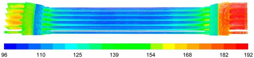
Processes 2019, 7, 256                                                                                2 of 15

     Typically, thermal analysis can be carried out using computational fluid dynamics (CFD) [6–8],
the heat equation finite element analysis (FEA) [4], or lumped parameter thermal network (LPTN)
models [9–11], and the first two are very accurate and deliver proper predictions of the thermal system
behavior during the component/device development. Finite volume method (FVM) is one of the
CFD methods and has the advantage of predicting the flow in complex regions and obtaining the
temperature distribution [8].
     With the development of high speed motors and their applications, the research and study of
the effect of different losses of motors have become topics of high interest. Luomi et al. [12] studied
and proposed a method for loss minimization including air-friction losses and explained that the
design is considerably influenced by the air-friction losses, resulting in a small diameter of the rotor.
Wang et al. [13] analyzed rotor losses of permanent magnet synchronous machine (PMSM) with
experiments and simulations and focused on rotor loss in the no load running condition. Aglen
and Andersson [14] theoretically and experimentally studied and calculated different losses of the
generator. They utilized a generator model to inspect the temperature distribution and showed that
different losses strongly affect the temperature distribution, particularly the temperature of the magnet
due to rotor losses. Leakage effects while proposing a design method for bearing were studied by
Le Yun et al. [15]. They discussed the effect of leakages in terms of static and dynamic stiffness. Zhang
and Kirtely et al. [16] investigated and predicted the power losses including core losses, winding losses,
and air-friction losses. The effects of friction loss in electric machines were often neglected in past
research; however, in recent years, the friction loss has been considered one of the important factors
that might affect the bearing life of the canned motor and account for the percentage of fly wheel loss
of the motor due to the increased rotational speeds. As in [12], a method for efficiency optimization of
a 500,000-r/min permanent magnet machine has been studied.
     There is no study on the friction loss and calculation method of the water-cooled canned motor
for the temperature rise of internal components and bearing safety. When the electric loss of the
motor is constant, the magnitude and calculation method of friction loss have an influence on the peak
temperature of the winding. The research object is a canned motor in this paper; a calculation method
is presented to study the effect of friction losses on the thermal field of the motor, and the effect on the
peak temperature and temperature variation characteristics of important parts are analyzed. The study
has been carried out by computational fluid dynamics (CFD) approaches adopting five friction loss
values: theoretical, experimental, assumed 1.1-times experimental, and the CFD module; the last one is
the ideal case assuming no friction loss.

2. Physical Model
     The studied electrical machine was a vertical squirrel cage motor with a rotational speed of
1500 r/min, 6600 kW (see Figure 1). It had a three-phase, four-pole, short-pitched, and double-layer
winding stator whose outside diameter was 1.3 m. The air gap clearance was 4.2 mm; the thickness of
the stator and rotor shield casing was 0.46 mm and 0.70 mm, respectively, and the dimensionless ratio
between core length and rotor inside diameter was 6.5. It had N-class insulation of the winding with a
permitted temperature of 200 ◦ C.
     In Figure 1, 1 indicates the outlet, 2 the upper nitrogen end room, 3 the water inlet, 4 the cooling
jacket, 5 the stator plate, 6 the upper radial bearing, 7 the stator core, 8 the winding end, 9 the frame,
10 the lower radial bearing, 11 the primary water inlet, 12 the lower fly wheel, 13 the axis, 14 the cage
rotor, and 15 the stator can.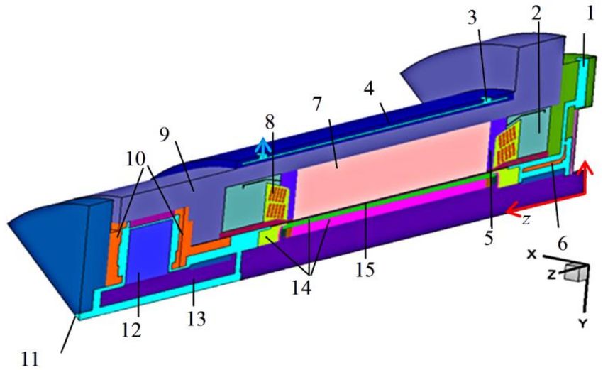
Processes 2019, 7, 256                                                                                     3 of 15

       Figure 1. Physical model of the computational domain showing different parts and flow directions.

     The temperature of each part can be reduced by the effective internal and external circuit design
of the primary cooling water. The secondary cooling water flowed from the upper part of the outer
casing (bottom outflow); see Figure 2. The primary water flowing out of the external heat exchanger
was drawn through the axial suction hole at the bottom of the frame. Water continued to flow upward
to the auxiliary impeller position and was thrown away by the Coriolis force. A part of the cooling
water flowed down for the cooling and lubrication of the lower guide bearing and lower fly wheel,
then entered into the cycle of cold water confluence and moved downward.

                          Figure 2. Schematic diagram of the water circulation circuit.

     Considering the continuity of flow of water in the shield, the geometry characteristics of rotor and
stator winding slots along the circumference, and the characteristics of heat transfer in stator and rotor
material, the 1/8th structure of the motor along circumferential direction was simulated. The rotor
shaft of the model was coincident with the z-coordinates; the positive direction of z-axis was towards
down, and the y-axis was positive along radial direction. The coordinate origin point was located in
the upper part and can be seen in Figure 1.
     In Figure 2, 1 indicates the primary water Inlet, 2 the flywheel clearance inert zone, 3 the lower
radial bearing clearance, 4 the auxiliary impeller position (confluence region), 5 the water in double
cans clearance, 6 the secondary water exit, 7 the secondary water inlet, 8 the upper radial bearing
clearance, and 9 the primary water outlet.

3. Solution Conditions

3.1. Basic Assumptions
1.     The water in the motor was an incompressible fluid because the Mach number (Ma = 0.24) was far
       less than 0.7. The mass flow rate (5.127 kg/s) of primary water was very large in the clearance of
       the motor. The Reynolds’s number (Re = 5363) showed that the flow was in the turbulence state.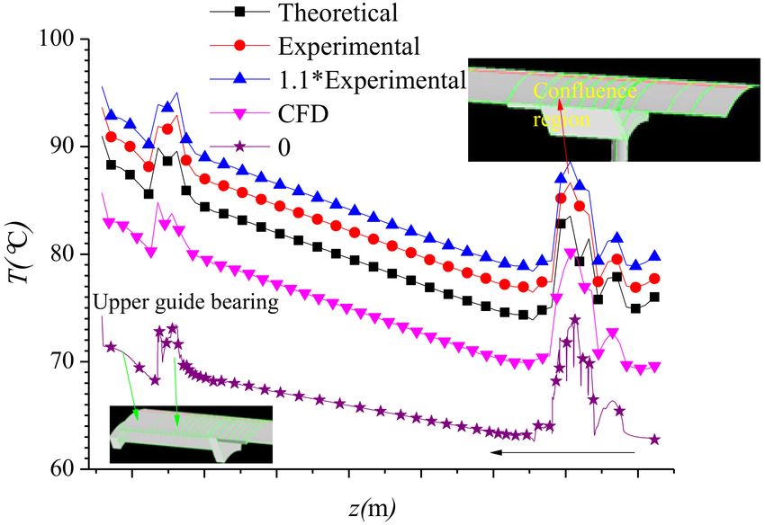
Processes 2019, 7, 256                                                                             4 of 15

2.    Only the steady state of fluid flow was considered. There was no contact thermal resistance
      between the adjacent bodies. The flow of the fluid in the internal passage was in the smooth region
      because the internal surface roughness of the wall in the motor was very small and the friction
      loss can be uniformly implemented for the corresponding positions of the water as volumetric
      heat sources inside the fluid.
3.    The electrical and harmonic losses and their distribution were calculated by another research
      institute using 3D software from the electromagnetic field. The corresponding loss in each
      body was uniformly distributed. Because the parameters of the thermo-physical properties of
      materials change with temperature variations, e.g., thermal conductivity, density, and specific
      heat at constant pressure, to be on the safe side, they were set as constant in the calculation
      process, so the minimum value of these parameters was chosen in the interval of the temperature
      through a large number of calculations. Among them, the thermal conductivity of the iron core
      lamination of rotor and stator was anisotropic, and the axial, radial, and tangential values of
      thermal conductivity were chosen experimentally. Except iron core lamination, other materials
      were isotropic, and their thermal conductivity values were selected conventionally.

3.2. Mathematical Model
     The rotation of the water in the shield sleeve gap and the water in the center of the axis was
considered in the calculation process because the rotor rotated rapidly relative to the stator under
the condition of stable operation. Therefore, a multiple reference-frame system and the rotational
speed of the wall surface were selected in the Ansys Fluent software (v14.5, Fluent Inc., New York, NY,
USA, 2012). Three-dimensional flow and heat transfer coupling equations including the mass and
momentum conservation equation and the relation of absolute velocity vector u (the velocity viewed
from the stationary frame) and relative velocity vector ur (the velocity viewed from the rotating frame)
can be written as follows:
                                                 ∇(ρur )                                             (1)

                          ∇(ρur ur ) + ρ(2Ω × ur + Ω × Ω × r) = −∇p + ∇τ + F)                         (2)

                                             u = ur + Ω × r                                           (3)

     In the fixed reference frame, mass, momentum, and energy conservation equations can be replaced
by a general control equation, which is given in Equation (4).

                                       ∇(ρu∅) = ∇(Γgradφ) + S                                         (4)

where Ω is the angular velocity of the rotor, φ is a universal variable, which can be replaced by
unknown variables u, v, w, T, etc., Γ is the generalized diffusion coefficient, and S is the generalized
source term. The only difference among the variables was the setting condition of Γ, S, initial values,
and boundary conditions. The specific expressions of Γ, S for different variables were provided in [16].
In addition, for the solid components in the motor, the energy equation was converted into the heat
conduction differential equation due to the no convection item. In the shielded motor, the mode of
heat transfer was conduction between and inside the solid materials (e.g., stator core), and between
the solid and liquid was the convection heat transfer. The natural convective heat transfer occurred
between the nitrogen and the adjacent solid wall surfaces at the end of the wire rod in the upper and
lower end closed room, and the magnitude of natural convection heat transfer was determined by the
temperature or density difference. The flow of water in the shielded casing and outer casing was a
mixed flow, and the natural convection in these regions can be neglected. Due to the small clearance
between the stator and rotor shield sleeve and in the three bearings, the width of flow was in the
order of millimeters. The forced convection flow in this region was affected by viscous shear stress
and Coriolis force, an effect whereby a mass moving in a rotation system experiences a force acting
perpendicular to the direction of motion and to the axis of rotation. Since a forced convection flow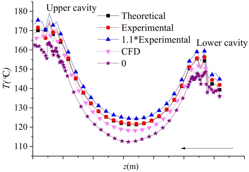
Processes 2019, 7, 256                                                                               5 of 15

around a cylinder is dominated by viscous shear forces in the boundary layer and the velocity gradient
between the walls is very large, so, in this paper, the shear stress transport (SST) k-ω two-equation
mathematical model was adopted. This model included two transport equations to represent the
turbulent properties of the flow. The first transported variable was turbulent kinetic energy k, and the
second transported variable was ω. These transported variables determined the energy in turbulence
and the scale of turbulence, respectively, and their equations can be written as follows:

                                  ∂             ∂      ∂k
                                                            !
                                     (ρkui ) =      Γk        + Gk − Yk + Sk                            (5)
                                 ∂xi           ∂x j    ∂x j

                              ∂             ∂      ∂ω
                                                        !
                                 (ρωui ) =      Γω        + Gω − Yω + Sω + Dω                           (6)
                             ∂xi           ∂x j    ∂x j
     In the above equations, Gk and Gω represent the generation of k and ω due to mean velocity
gradients. Γk and Γω represent the effective diffusivity of k and ω, respectively. Yk and Yω represent
the dissipation of k and ω due to turbulence. Dω represents the cross-diffusion term. Sk and Sω are
user-defined source terms [17].

3.3. Mesh Generation
     Due to the complex geometry of the model, both structured and unstructured meshes were used,
while the total number of cells was 14,099,447, and the value of equisized skew was less than 0.8 for
the overall mesh. The mesh was refined into those regions where large velocity and pressure gradients
were expected. In this paper, the grid independence solution was obtained after employing different
meshing schemes, interval sizes, and calculations.

3.4. Loss and Boundary Conditions

3.4.1. Water Friction Loss
      There were losses that caused the temperature rise in the motor, and in this paper, only water
friction loss and relative influencing factors were given more attention. Principally, friction loss can be
divided into loss along the path and local losses. The losses along the path were due to the frictional
resistance caused by the fluid moving along the flow path and occurred in the fluid boundary layer
where the velocity gradient was comparatively large. Local losses were due to fluid flow through
various curved pipelines, for example, in elbows, valves, etc., due to the deformation of water flow,
the change of direction, and speed redistribution, and the internal eddy current caused losses. The
loss along the path was caused by viscous friction, and the frictional resistance coefficient was closely
related to the surface roughness of the water channel, the state of flow, and the properties of the coolant.
      In this paper, the value of surface roughness for each method was set the same. The analysis
of friction losses in the water gap clearance can be estimated by the equation derived for rotating
cylinders, which can be written as [18,19]:

                                              P = kc f πρΩ3 r4                                          (7)

where k is the roughness coefficient, where the value was 1.0 for smooth surface [4], ρ is the density
of water, l is the length of the cylinder, and r is the rotor radius. The friction coefficient cf depends
on the radius of the cylinder, the radial air-gap length δ, and the Reynolds number. The calculated
result of the water friction loss at every clearance position of the water channel can be seen in Table 1.
In order to verify the accuracy of the calculation results, a friction loss experiment was also carried out.
The experimental loss value was obtained by the loss-separation method [18] and was provided by
the manufacturer.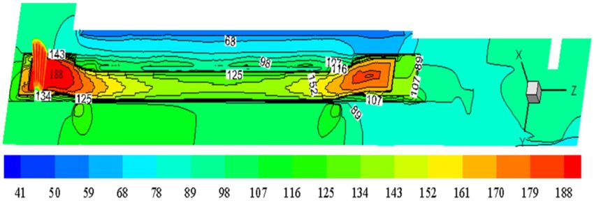
Processes 2019, 7, 256                                                                                                6 of 15

        Table 1. Four conditions of friction losses (kW) at different positions in the water clearance region.

       Clearance Position          Assumed Value           Analysis Value             Test Value      Assumed Value
         Shield sleeve                     0                      384                    407             407 × 1.1%
      Upper radial bearing                 0                       17                     17              17 × 1.1%
      Lower radial bearing                 0                       17                    17               17 × 1.1%
        Upper fly wheel                    0                      793                   722              722 × 1.1%
        Lower fly wheel                    0                      580                    690             690 × 1.1%
        Auxiliary wheel                    0                        7                      7               7 × 1.1%
             Total                         0                     1798                   1860                 2046
                  Note: The data in the Table 1 are the sum of local and along-the-way losses at each location.

      Table 1 shows that the analysis value of the water friction loss in the water clearance (region) of
the lower fly wheel and double cans was smaller than that of the test value by 110 kW and 23 kW,
respectively, and of the upper flywheel was larger than the test value by 71 kW. Analysis of friction
loss was smaller than the experimental friction loss by 62 kW, a relative difference of −3.33%; hence,
the results were accurate (the total experimental friction loss was large). Based on previous experience
and for the sake of operational safety, it was assumed that the actual operating condition (value) was
higher than the test value by 10% in every term. The values of analysis and experimental water friction
loss at each position were provided by the manufacturer; see Table 1. In order to separate the influence
of water friction loss on temperature rise, a situation in which the water friction loss was assumed as
zero was designed, as shown in the Table 1.
      It was assumed that the friction losses at each location was evenly distributed. The value of water
friction loss per unit volume as a source term (kW/m3 ) was calculated according to Table 1, and these
values were applied to the corresponding boundary volume of water, respectively. The CFD method
was different from the above-mentioned conditions in Table 1. The friction loss in the clearance of
water at different positions was calculated by the CFD FLUENT software. The specific way of selecting
the viscous heating item was to select it in the “options” list, which is right under the turbulence model,
and the wall roughness was set in the boundary conditions according to the different positions of the
cans. All the related settings and parameters used in the CFD models above calculations are listed in
Table 2. We can see the differences between the two calculation methods of water fiction loss.

      Table 2. The settings and parameters in the computational fluid dynamics (CFD) models for temperature
      calculations. SST, shear stress transport.

                                               CFD          Assumed          Analysis      Test     Assumed Value
         Models-viscous-(SST) k-ω              on               on              on          on              on
              Models-energy                    on               on              on          on              on
          Options-viscous heating              on               off             off         off             off
                 Boundary
                                               set               -               -             -             -
          condition-moving wall
              Shear condition               no slip              -               -             -             -
           Wall roughness (mm)                1.0                -               -             -             -
            Source item in water
                                                -                -              on          on              on
         clearance region (kW/m3 )
                                          Note: “-” denotes no need to set any value.

3.4.2. Electrical Loss
     The electric loss in the rotor was calculated in the iron core, the shield sleeve, the end of the
coupling loop, and in the copper bar. Harmonic loss of the wire rod was also a part of this calculation.
The electric loss in stator was calculated in the shield sleeve, the copper bar, and in the iron core.
In particular, the stator and rotor core teeth and yoke loss were calculated separately, and the teeth
were divided into 16 sections along the radial direction. In addition, the loss value of the conical ring,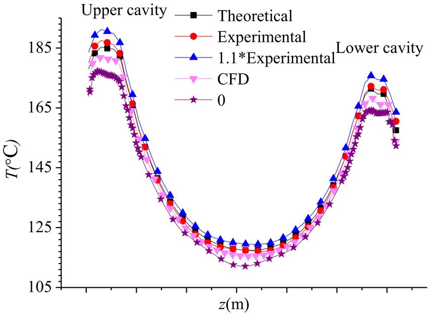
Processes 2019, 7, 256                                                                              7 of 15

teeth, and yoke position of the stator finger plate was considered. The stray loss was calculated by the
experimental formula developed by the factory for the same kind of shield motor. By using the same
loss calculation method as used in [3], the obtained calculated values of the main parts were as given
in Table 3.

                         Table 3. Electrical loss values in the main solid components.

                                       Components                        Loss (kW)
                                     Rotor copper bar                        72.0
                                   Rotor shield (casing)                   262.57
                                      Stator winding                        44.54
                                   Stator shield (casing)                  920.58
                                       Conical ring                         28.53

     It can be noted from the above table that the electrical loss was comparatively more in the rotor
and stator shielding case. It was assumed that all electrical losses were distributed uniformly in the
corresponding components.

3.4.3. Boundary Conditions
      The inlet boundary condition of the volume flow rate of water was mainly determined by the
intersection point of the pump and motor operating curves and partially determined by the geometry
characteristics. The entrance of the primary water below the base and the entrance of the external
cooling water in the upper part of the shielding casing (see Figure 2) were the velocity boundary
conditions, and the magnitude of velocity was set experimentally. The rated rotating speed of the
motor shaft was 1500 r/min.
      The inlet-outlet temperature of the primary water was closely related to factors such as the
magnitude of internal friction loss, the temperature of cooling water in the external heat exchanger
(same as the secondary water temperature in the cooling jacket), and the velocity of water. Through
the calculation of the heat balance and heat transfer of the internal motor and external heat exchanger,
respectively, and between the internal motor and external heat exchanger, at the operating condition of
the highest external cooling water temperature of 41 ◦ C at entrance, we obtained the internal cooling
water inlet temperatures, 60.38 ◦ C, 61.65 ◦ C, and 62.99 ◦ C, at the three mentioned conditions. For the
convenience of comparison, the temperature of the internal water inlet was set at the same temperature
of 60.38 ◦ C.
      The gauge pressure at the outlet of the external water was set to 0 Pa. The mode of heat transfer
in the outer surface of the shell was natural convection. For safety measures, the surface convective
heat transfer coefficient was set to 1 W (m2 K), and the ambient air temperature of the outer surface
was 48.9 ◦ C. The boundary condition at the top of the motor was constant heat flux, and its value was
water friction loss per unit volume at the bottom fluid of the flywheel. The boundary conditions of the
right and left surface of the calculation domain (see Figure 1) were linked periodically. In addition, the
governing equations for the fluid and solid regions were solved by using FLUENT 14.5, which uses
the finite volume method. A second order upwind scheme was employed for the discretization of
all the variables, and the simple scheme was used for the pressure-velocity coupling. The standard
wall function was used to deal with the viscosity lamination near the solid wall surface, and the
dimensionless distance y+ met the requirements. After trying several different mesh topologies and
sizes, the grid-independent solution was obtained.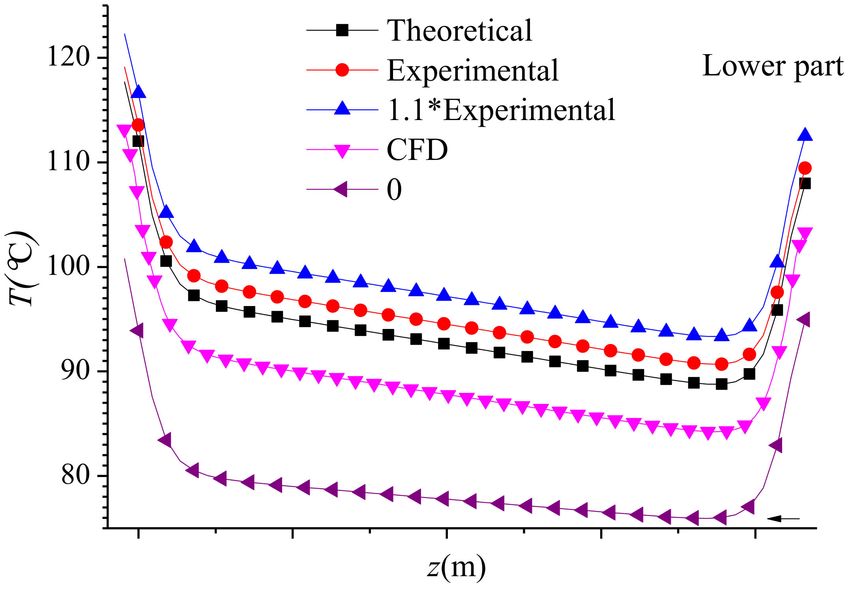
Processes 2019, 7, 256 8 of 15
4. Results and Discussion
The temperature field in the solution domain was obtained by means of numerical simulation of
Equations (1)–(6) at the loss and boundary conditions mentioned above.
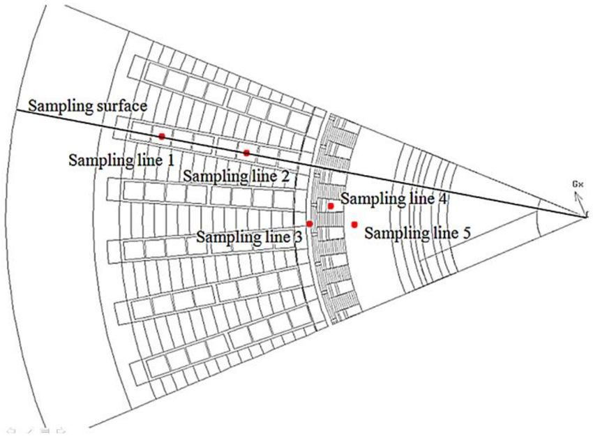
For the convenience of analysis, five straight lines (sampling lines) parallel to the rotation axis
were drawn in order to get the axial variation law of physical quantity. The position of each line is
shown in Figure 3, and the number of sampling lines required for the analysis is given in decreasing
order of radii. The sampling surface was located at the radial cross-section of the stator slot; Sampling
Lines 1 and 2 pass through the center of the stator lower and upper winding, respectively, and the
start and end coordinates of the two lines are the same. Sampling Line 3 is located in the center of
the clearance of the cooling water between the stator and rotor shield, and Sampling Lines 4 and 5
pass through the center of a rotor bar and the rotor core, respectively. This paper presents the analysis
of the effect of water friction loss on the temperature of canned motor components such as the stator
winding, rotor copper bar, rotor iron core, and on the internal water passage. The temperature analysis
of different parts is described below.
Figure 3. Position of sampling lines and the surface in cross-section.
4.1. Temperature Analysis of the Stator Winding
The temperature distribution characteristics of the stator winding were the same in the axial
direction, and the highest temperature point was located in the middle of the nose of the two ends
of the stator winding (see Figure 4), resulting in a reduction of the heat by the conduction from the
two ends of the stator to the middle, and was then delivered by the primary and secondary water
convection. The position of peak temperature was not changed when calculated for four different
conditions; assuming no fiction loss, analysis, experimental, and assuming 1.1-times the experimental
value. The peak temperature increased gradually by 178.6 ◦ C, 185.8 ◦ C, 188.2 ◦ C, and 192.0 ◦ C, and the
maximum temperature did not exceed the permitted temperature of 200 ◦ C, i.e., no over-temperature.
Processes 2019, 7, 256                                                                                     9 of 15

      Figure 4. Temperature contour of the stator winding for the assumed maximum friction loss
      condition (◦ C).

      The results showed that electrical loss was the main factor that rose the temperature of the winding,
although the total value of the analysis of water friction loss was comparatively higher, but did not
strongly affect the peak value of the temperature. Comparing it (peak temperature) with the no fiction
loss condition, its temperature value increased by 7.2 ◦ C, 9.6 ◦ C, and 13.4 ◦ C, and it showed that if the
mechanical loss of water friction was neglected, the error would be about 10 ◦ C. Comparing it (peak
temperature) with the experimental calculation of the water friction loss condition, its temperature
value increased by −2.4 ◦ C and 3.8 ◦ C, and the error was within the range ±2.0%, while the values of
peak temperature increased non-linearly. The temperature contour of the stator winding at assumed
1.1-times the experimental calculation condition of water friction loss (maximum friction loss) is given
in Figure 4.
      In order to analyze the influence of water friction loss calculation methods on the temperature
field of the motor, using the same conditions mentioned above and the CFD module, the obtained
results showed that the peak temperature of the motor winding was 180.9 ◦ C, and comparing with the
experimental water friction loss values, it reduced by 7.93 ◦ C (error was −3.84.2%), while temperature
distribution characteristics and peak position did not change. The value of temperature was lower
when calculated by the CFD module. The main cause of the error was that the actual wall roughness
was higher than 1.0 mm.
      It can be seen from Figure 4 that the peak temperature of the end center of the stator winding
nose in the upper nitrogen end room was 192.0 ◦ C. The highest temperature of stator winding in the
lower nitrogen end room was lower than that in the upper part. The temperature of the winding
adjacent to the central part of the iron core was lower because the surrounding water temperature in
the internal gap and in external casing was lower and the convection heat transfer capability of the
water was strong.
      Figure 5 shows the temperature contour on the sampling surface for the test calculated condition.
Theoretically, the temperature distribution characteristics on the surface of any polar angle along the
circumferential cross-section are a typical case. The overall temperature distribution characteristics
of any component along the radial direction can be seen in Figure 5. The temperature of the casing
near the cooling water zones was low. Secondly, the temperature of the water in the stator and rotor
shield sleeve clearance, stator iron core, and the rotor was higher; the stator winding temperature in
the upper nitrogen chamber was the highest; and the temperature gradient near the tooth clamp plate
was relatively large.

               Figure 5. Temperature distribution of the radial sampling surface at a polar angle (◦ C).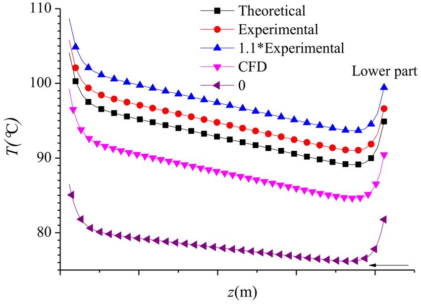
Processes 2019, 7, 256                                                                                  10 of 15

      Figures 6 and 7 show the temperature distribution of Sampling Lines 1 and 2 of the stator winding
along the z-axis, respectively. From Figures 6 and 7, it can be seen that the temperature distribution
of the winding presented a concave curve, and the lowest temperature point in the upper and lower
windings was near the axial center of the windings. Ignoring frictional losses, the temperature rise
caused by electric loss was shown in the curve corresponding to “0” in the figure, and this curve can be
used as a benchmark for comparison. In comparison, it can be found that the temperature rise of the
winding due to frictional loss at the upper and lower ends and the intermediate position was larger.
It is one of the main purposes of this paper to reveal the influence of friction loss on the calculation
of peak temperature. Except for the cavity at both ends, for the theoretical and experimental friction
losses, the temperature distribution curve was basically coincident.

              Figure 6. Temperature distribution of the lower part of stator winding Sampling Line 1.

              Figure 7. Temperature distribution of the upper part of stator winding Sampling Line 2.

     The temperature distribution of the winding was not symmetrical along the axial center of the
iron core. The temperature gradient in the left part of the winding was higher than that in the right
part of the winding, and the winding temperature in the upper stator cavity was higher than that of
the lower stator cavity. In the same z-coordinates, the temperature of Sampling Line 1 of the lower
winding was higher than the temperature of Sampling Line 2. For Sampling Line 2, where the upper
winding location was closer to the shaft, the actual length of the winding nose was short in the upper
and lower part of the stator cavity.
Processes 2019, 7, 256 11 of 15
In Figure 7, the irregular variation of the curve indicates the change of temperature in insulation,
nitrogen (end room), and other parts through which the sampling line passed after stretching out the
straight winding. Under conditions of analysis of and experimental water friction loss, the temperature
of the winding was basically the same for the same position, except the end cavity. However, for
the two end stator cavities, the calculation results were different in the five cases. The value of the
winding temperature was the highest at the same position along the z-axis, under the water friction loss
condition of 1.1-times the experimental value, and was lowest when calculated by the CFD module.
4.2. Temperature Analysis of the Primary Water Passage
Figure 8 shows the temperature distribution of Sampling Line 3 in the internal water passage
between the stator and rotor shield. It can be seen from Figure 2 that Sampling Line 3, in turn, through
the water clearance at the position of the upper guide bearing, double cans, near the confluence region,
and approximately no water flowing area at the bottom of the lower flywheel, increased in the direction
of the z-axis. The annular cross-sectional area of water in the confluence region became larger, whereas
in the other region, the cross-sectional width was in mm.
Figure 8. Temperature distribution of water passage Sampling Line 3 along the z-axis.
It can be seen in Figure 8 that the temperature of water rise was linear between the double cans
region, and the cross-sectional area of water was the same. The maximum water temperature value for
the four conditions of water friction loss was no more than the alarm temperature of 90 ◦ C; however,
the calculation results of the position of the upper guide bearing were inconsistent. The frictional loss
did not exceed the temperature when calculated using CFD and the theoretical method, but in the
other two cases, local temperature exceeded the rated condition. This example shows that the different
calculation methods of friction loss had an influence on the conclusion about whether the water of
the upper guide bearing was over temperature or not. It can provide a reference for the design of the
internal water passage. The average temperature of water corresponding to the experimental friction
loss value of Sampling Line 3 was higher by 2.6 ◦ C than that of the analysis value calculated at the
same position, and was lower by about 2.0 ◦ C than the assumed value. For the CFD case, the average
value of the temperature of Sampling Line 3 was lower by about 4.8 ◦ C than that of the analysis value
calculated at the same position. The average temperature of the water was 8.2 ◦ C higher than that
without friction loss.
The sudden rise of the temperature of two local positions is indicated in Figure 8. In the clearance
(gap) of the upper guide bearing, the temperature of the water increased linearly, and the temperature
of the water near the exit, at the bottom of the upper flywheel, increased dramatically due to the heat
source in it. In the water clearance near the confluence region, there was an approximately no waterProcesses 2019, 7, 256 12 of 15
flow region, so a lower rate of heat transfer was in this area. The water temperature was higher than
that of the inlet of the rotor shield sleeve.
4.3. Temperature Analysis of the Rotor Copper Bar
Figure 9 shows the temperature variations of the sampling line of the rotor copper bar along
the z-axis for the five conditions of water friction losses. It shows that the temperature distribution
characteristics of the rotor cooper bar were different from the stator winding mentioned above in
Figures 6 and 7. The temperature of the rotor copper strip at the lower and upper end loop position
rose dramatically, and the temperature gradient was larger because there was a large heat source of
electrical loss in the end ring.
Figure 9. Temperature distribution of rotor copper bar Sampling Line 4.
The average temperature of the rotor copper bar of Sampling Line 4 corresponding to the analysis
of friction loss value was lower by about 1.9 ◦ C and 4.5 ◦ C than that by the experimental value and by
assuming 1.1-times the experimental value, respectively, and when friction losses were ignored, it was
lower by 14.82 ◦ C than that corresponding to the analysis of the friction loss value. The value of the
average temperature of Sampling Line 4 was lower by about 4.71 ◦ C than that of the calculated analysis
value, when calculated by the CFD module. It shows that the large friction loss had a relatively large
influence on the temperature rise of the rotor bar.
4.4. Temperature Analysis of the Rotor Iron Core
Figure 10 shows the temperature variations of Sampling Line 5 of the rotor iron core tooth along
the z-axis for the five conditions of water friction losses, and it can be seen that the temperature
distribution characteristics of rotor iron core were similar to Figure 9, different from Figures 6 and 7.
There was a sharp rise in the local temperature gradient due to large electric loss in the tooth plate and
in the end ring that were located in the lower and upper end of the rotor core, and the temperature
distribution of the rotor iron core tooth changed linearly in the double cans section. The temperature
of the rotor iron core also gradually increased, and the characteristics were the same as mentioned in
the above Figure 9, while only the peak value was different.
It can be concluded that the characteristics of the temperature distribution curves did not change
when the calculating method of water friction loss changed (as can be seen in Figures 6–10), and the
value of the temperature (in Figures 8–10) was the highest at the same position under the water friction
loss condition of 1.1-times the experimental value and lowest when calculated by the CFD module.Processes 2019, 7, 256 13 of 15
Figure 10. Temperature distribution (◦ C) of rotor core Sampling Line 5.
4.5. Accuracy Analysis of Temperature Calculation Results
The temperature calculations obtained at different water friction loss conditions had very small
differences from each other. The position of peak temperature corresponding to the analysis value of
the loss was same, but the peak value difference was −1.2 ◦ C, when compared with the result of the
earlier finite difference method software, which was developed by the factory.
Additionally, under the no load operating condition, multi-point temperature measurement had
been performed. To verify the accuracy of the calculation results, the same numerical method (the
water friction loss per unit volume was set as heat sources in the corresponding clearance of water)
was adopted to calculate the temperature field under the no-load test condition. The error in the
temperature results on the many positions simulated (using the method mentioned above) was 5%
lower than the test values. However, at present, the thermal test of the motor in the fully-loaded
condition has not yet been performed.
The results in this paper were accurate and satisfied the engineering requirements.
5. Conclusions
In this paper, a canned motor has been taken as an example, and a method was presented to study
the effect of friction losses on the calculation of the thermal field of the motor using the CFD FLUENT
software, that is: the water friction loss per unit volume was added in the corresponding position
as the heat source; the viscous heating item option was kept inactive; and the wall roughness in the
boundary conditions was not set. For the second method, the friction losses was calculated by the CFD
FLUENT software, whereby the option of the viscous heating item was selected, which is right under
the turbulence model list, and the wall roughness in the boundary conditions was set according to the
different positions of the cans. The conclusion are as follows:
1. The peak temperature of the motor winding was lower by −4.2% as compared to the water
friction loss calculated by CFD with the proposed water friction loss per unit volume method.
This method of, i.e., using given experimental water friction loss per unit volume as the source
term did not change the characteristics of the temperature distribution of the components of the
motor and intercooling water.
2. The temperature along the axial direction increased with the increase of friction loss at the same
position of the rotor copper bar, rotor iron core, and for water in the clearance of double cans, and
the tendency of the temperature distribution increased linearly along the axial direction where
the shield was located.
3. The temperature distribution of the winding presented a concave curve, and the lowest
temperature point in the upper and lower winding was near the axial center of the winding.Processes 2019, 7, 256 14 of 15
4. For the water-cooled shielded motor, the water friction loss cannot be ignored. The calculation
method of the water friction loss had a great influence on the conclusion about whether the water
of the upper guide bearing was over temperature.
Author Contributions: Y.L. and A.M. are the main authors of this manuscript. All the authors contributed to
this manuscript. All authors read and approved the final manuscript. Y.L. and A.M. conceived of the novel idea
and performed the analysis; A.M. and Y.L. analyzed the data; A.M. and Y.L. contributed analysis tools; A.M. and
Y.L. wrote the entire paper; M.A.R., S.R., S.A., M.S., and A.W.A. checked, reviewed, and revised the paper. Y.L.
performed the final proofreading and supervised this research.
Funding: This research received no external funding.
Conflicts of Interest: The authors declare no conflict of interest.
References
1. Boglietti, A.; Cavagnino, A. Evolution and modern approaches for thermal analysis of electrical machines.
IEEE Trans. Ind. Electron. 2009, 56, 871–882. [CrossRef]
2. Yetgin, A.G. Effects of induction motor end ring faults on motor performance. Experimental results.
Eng. Fail. Anal. 2009, 96, 374–383. [CrossRef]
3. Liang, Y.; Bian, X.; Yu, H.; Li, C. Finite-element evaluation and eddy-current loss decrease in stator end
metallic parts of a large double-canned induction motor. IEEE Trans. Ind. Electron. 2015, 62, 6779–6785.
[CrossRef]
4. Huang, Z.; Fang, J.; Liu, X.; Han, B. Loss calculation and thermal analysis of rotors supported by active
magnetic bearings for high-speed permanent-magnet electrical machines. IEEE Trans. Ind. Electron. 2016, 63,
2027–2035. [CrossRef]
5. Chiu, H.C.; Jang, J.H.; Yan, W.M.; Shiao, R.B. Thermal performance analysis of a 30 kW switched reluctance
motor. Int. J. Heat Mass Tran. 2017, 114, 145–154. [CrossRef]
6. Kim, C.; Lee, K.S. Thermal nexus model for the thermal characteristic analysis of an open-type air-cooled
induction motor. Appl. Therm. Eng. 2017, 112, 1108–1116. [CrossRef]
7. Kim, C.; Lee, K.S. Numerical investigation of the air-gap flow heating phenomena in large-capacity induction
motors. Int. J. Heat Mass Tran. 2017, 110, 746–752. [CrossRef]
8. Lu, Y.; Liu, L.; Zhang, D. Simulation and analysis of thermal fields of rotor multislots for nonsalient-pole
motor. IEEE Trans. Ind. Electron. 2015, 62, 7678–7686. [CrossRef]
9. Lancial, N.; Torriano, F.; Beaubert, F.; Harmand, S.; Rolland, G. Study of a Taylor-Couette-Poiseuille flow
in an annular channel with a slotted rotor. In Proceedings of the International Conference on Electrical
Machines (ICEM), Hangzhou, China, 2–5 September 2014; pp. 1422–1429.
10. Traxler-Samek, G.; Zickermann, R.; Schwery, A. Cooling airflow, losses, and temperatures in large air-cooled
synchronous machines. IEEE Trans. Ind. Electron. 2010, 57, 172–180. [CrossRef]
11. Tu, J.; Yeoh, G.H.; Liu, C. Computational Fluid Dynamics: A Practical Approach, 3rd ed.; Butterworth-Heinemann:
Oxford, UK, 2018.
12. Luomi, J.; Zwyssig, C.; Looser, A.; Kolar, J.W. Efficiency optimization of a 100-W 500,000-r/min
permanent-magnet machine including air-friction losses. IEEE Trans. Ind. Appl. 2009, 45, 1368–1377.
[CrossRef]
13. Gengji, W.; Ping, W. Rotor loss analysis of PMSM in flywheel energy storage system as uninterruptable
power supply. IEEE Trans. Appl. Superconduct. 2016, 26, 1–5. [CrossRef]
14. Aglen, O.; Andersson, A. Thermal analysis of a high-speed generator. In Proceedings of the 38th IAS
Annual Meeting on Conference Record of the Industry Applications Conference, Salt Lake City, UT, USA,
12–16 October 2003; Volume 1, pp. 547–554.
15. Le, Y.; Sun, J.; Han, B. Modeling and design of 3-DOF magnetic bearing for high-speed motor including
eddy-current effects and leakage effects. IEEE Trans. Ind. Electron. 2016, 63, 3656–3665. [CrossRef]
16. Zhang, F.; Du, G.; Wang, T.; Wang, F.; Cao, W.; Kirtley, J.L. Electromagnetic design and loss calculations of a
1.12-MW high-speed permanent-magnet motor for compressor applications. IEEE Trans. Energy Convers.
2016, 31, 132–140. [CrossRef]
17. Lomax, H.; Pulliam, T.H.; Zingg, D.W. Fundamentals of Computational Fluid Dynamics, 1st ed.; Springer Science
& Business Media: Berlin, Germany, 2013.Processes 2019, 7, 256 15 of 15
18. Heins, G.; Ionel, D.M.; Patterson, D.; Stretz, S.; Thiele, M. Combined experimental and numerical method
for loss separation in permanent-magnet brushless machines. IEEE Trans. Ind. Appl. 2016, 52, 1405–1412.
[CrossRef]
19. Saari, J. Thermal Analysis of High-Speed Induction Machines. Ph.D. Dissertation, Department of Electrical
and Communications Engineering, Helsinki University of Technology, Espoo, Finland, 1998.
© 2019 by the authors. Licensee MDPI, Basel, Switzerland. This article is an open access
article distributed under the terms and conditions of the Creative Commons Attribution
(CC BY) license (http://creativecommons.org/licenses/by/4.0/).You can also read