GCMs Derived Projection of Precipitation and Analysis of Spatio-Temporal Variation over N-W Himalayan Region
←
→
Page content transcription
If your browser does not render page correctly, please read the page content below
August 2015                                                                                             1

GCMs Derived Projection of Precipitation and
Analysis of Spatio-Temporal Variation over
N-W Himalayan Region
Dharmaveer Singh*1, R.D. Gupta2 and Sanjay K. Jain3
1
  GIS Cell, Motilal Nehru National Institute of Technology Allahabad- 211004, India
2
  Department of Civil Engineering, Motilal Nehru National Institute of Technology, Allahabad-
  211004, Uttar Pradesh, India.
3
  Scientist-F, Water Resources Systems Division, National Institute of Hydrology, Roorkee- 247667,
  India.

   ABSTRACT
   The ensembles of two Global Climate Models (GCMs) namely, third generation Canadian Coupled
   Global Climate Model (CGCM3) and Hadley Center Coupled Model, version 3 (HadCM3) are
   used to project future precipitation in a part of North-Western (N-W) Himalayan region, India.
   Statistical downscaling method is used to downscale and generate future scenarios of precipitation
   at station scale from large scale climate variables obtained from GCMs. The observed historical
   precipitation data has been collected for three metrological stations, namely, Rampur, Sunni and
   Kasol falling in the basin for further analysis. The future trends and patterns in precipitation
   under scenarios A2 and A1B for CGCM3 model, and A2 and B2 for HadCM3 model are analyzed
   for these stations under three different time periods: 2020’s, 2050’s and 2080’s. An overall rise
   in mean annual precipitation under scenarios A2 and A1B for CGCM3 model have been noticed
   for future periods: 2020’s, 2050’s and 2080’s. Decrease, in precipitation has been found under
   A2 and B2 scenarios of HadCM3 model for 2050’s and slight increase for 2080’s periods. Based
   on the analysis of results, CGCM3 model has been found better for simulation of precipitation in
   comparison to HadCM3 model.
              Keywords: CGCM3, HadCM3, Statistical downscaling method, Precipitation

1. INTRODUCTION                                       change may amend availability of water along
                                                      with the risk of increased frequency of droughts
Availability of abundant water on time is a
                                                      and floods (Kumar and Jain 2010). The proper
prime concern for agriculture, energy and
                                                      assessment of potential water resources is
industrial sectors in India. The country has
                                                      required in order to maintain continuous water
viewed increase in demand of water due to rapid
                                                      supply to various sectors such as agricultural,
growth in population and economy. Studies by
                                                      industrial, energy and domestic in future
various authors show that change in patterns of
                                                      (Gosain et al., 2011).
temperature and precipitation due to climate
* Corresponding author : Dharmaveer Singh, E-mail:veermnnnit@gmail.com

Journal of Hydrology and Meteorology, Vol. 9, No. 1                                     SOHAM-Nepal
2 GCMs Derived Projection of Precipitation and Analysis ... August 2015 Precipitation determines the magnitude of of the order 50,000km2) spatial resolution available water and is an important factor. (Xu.,1999). This limits the direct applications Knowledge about past and future precipitation of GCM’s outputs in regional climate change along with its variability has scientific as well as impact studies (Ghosh, 2010; Raghavan et practical significance in climate change impact al., 2012; Wilby et al., 2002). A methodology studies. Investigating how change in climate usually known as downscaling is introduced for will alter future precipitation and its spatial and bridging the gap between the scale of GCMs and temporal variability is an area of active research required resolution for practical applications. (Basistha et al., 2009). Generally, assessment Downscaling methodology broadly can be of likely future precipitation is done under a classified into statistical and dynamical methods climate change scenario (Anandhi et al., 2008). (Ghosh, 2010). A climate scenario which refers to plausible Statistical downscaling method is supported by future climate is a time series of synthetic the view; the regional climate is conditioned weather data. These scenarios are based on by large scale climate state and regional/local future emission of greenhouse gases and used to physiographic features (e.g. topography, land- study possible effects of human-induced climate sea distribution and land use/land cover). In change (Lapp et al., 2009). Uncertainties this method, large scale atmospheric variables associated with scenarios are an important issue (predictors) of GCMs are related to station- in scientific communities as it is very intricate scale climate variables (predictands) based on to determine nature of future concentrations empirical relationship (Kim et al., 1984; Raje of greenhouse gasses in atmosphere based on and Mujumdar, 2011; von Storch et al., 2000). anthropogenic activities (Carter et al., 2001). The statistical downscaling methods can be Scenarios should not be taken as forecasts of classified into 3 categories; weather typing, future climate as these are constructed to provide weather generator and regression method (Wilby sufficient quantitative measures of uncertainty and Wigley, 1997). In literature, the strength and represented with a range of plausible future weakness of each method is critically analyzed paths (Lapp et al., 2009). Anandhi et al. (2008) (Bárdossy et al., 2005; Dubrovsky et al., 2004; has strongly advocated for using a range of Fowler et al., 2000; Hua et al., 2010; Kilsby et scenarios in climate change impact studies. al., 2007; Mason, 2004; Tripathi et al., 2006 Global Climate Models (GCMs), the most Wilby et al., 1999). In dynamical downscaling credible available tools, are used to simulate method physical processes are simulated at fine state of the present and future climate using scale from host GCMs using a Regional Climate transient climate simulations. In a transient Model (RCM). A horizontal resolution of the simulation, anthropogenic forcings, decided on order of tens of kilometers is obtained from the basis of IPCC climate scenarios, are changed RCMs over selected area of interests. RCMs gradually in a realistic fashion (Anandhi et al, accounts use of initial boundary conditions 2008). The decrease in the accuracy of GCMs and time dependant lateral meteorological simulated climate variables has been observed conditions derived from GCMs to provide from continental to local scale as they are information at high spatial and temporal scales unable to capture sub-grid scale features and (Giorgi, 1990; Jones et al., 1995). The complex physical dynamics due to their coarse (typically design and computationally expensive nature of Journal of Hydrology and Meteorology, Vol. 9, No. 1 SOHAM-Nepal
August 2015                Dharmaveer Singh, R.D. Gupta & Sanjay K. Jain                              3

RCMs has limited their applications in climate        modelled projections have shown a decrease
change impact studies (Ghosh and Mishra,              of about 20% in monsoon precipitation in
2010; Hewitson and Crane 1996).                       most parts of Pakistan and in south-eastern
                                                      Afghanistan by the end of the century. The
The Himalayan mountain systems which are
                                                      Tibetan plateau will exhibit increase (10–30%)
birth place of many perennial river systems such
                                                      in mean annual precipitation by 2080 (IPCC,
as the Indus, the Ganga and the Brahmaputra
                                                      2007). Rupa Kumar et al. (2006) observed
have also a strong influence over the climate of
                                                      projected increase of 20 to 30% in precipitation
Indian sub-continent (Bhutiyani et al., 2007).
                                                      for the western Himalayan region by the end of
Hence, a small change in the climate of the
                                                      21st century.
Himalaya has a potential to bring devastating
effects on the socio-economic survival of             Keeping the above in mind, the objective of
millions of people living in these basins. Jain       the present paper is to study the change in
(2012) observed that trend analysis of past           patterns of future precipitation under various
precipitation data in India has not revealed any      emission scenarios over North-Western (N-
significant extensive change in the patterns          W) Himalayan region, India. For this purpose,
so far, but the simulated results derived from        a software called Statistical Downscaling
GCMs illustrate that in future these patterns are     Model version 4.2 (SDSM 4.2) is used for
likely to change. These changes would not be          downscaling of precipitation from large
uniform over space and time domain as some            scale climate predictors obtained from third
areas are expected to receive more precipitation      generation Canadian Coupled Global Climate
and others less. There may be increase in             Model (CGCM3) and Hadley Center Coupled
frequency of extreme precipitation events.            Model, version 3 (HadCM3). India. SDSM
Similar trend in precipitation has also been          4.2 is used to generate single-sites scenarios of
detected over Himalayan region. The north-            daily surface weather variables from large scale
east region along with eastern and central parts      climate predictors simulated by GCMs (Wilby
of the Tibetan Plateau has reveled increasing         et al., 2007). The future patterns and variability
trend in annual precipitation while the western       in precipitation under scenarios A2 and A1B for
Tibetan region shows decreasing trend (Zhao et        CGCM3 model, and A2 and B2 for HadCM3
al., 2004; Xu et al., 2008). Similarly, the north-    model are analyzed under three different time
western Himalayan region (northern Pakistan)          periods: 2020’s (2011-2040), 2050’s (2041-
has experienced an increasing trend while Nepal       2070) and 2080’s(2071-2099).
exhibited no long-term trend in precipitation
(Farooq and Khan, 2004; Shrestha et al., 2000).
                                                      2. STUDY AREA
Increase in post-monsoon precipitation has
been detected at Dehradun, Pithoragarh and            The study area is a part of the Sutlej river basin
other western Himalayan stations whereas              and confined to the State of Himanchal Pradesh,
decrease in winter (Pant et al., 1999). Kumar et      India. The State shares its boundary with four
al. (2005) found an increasing trend in annual        Indian States namely, Jammu and Kashmir
precipitation but decreasing trend in monsoon         from North, Punjab from West, Haryana from
precipitation over Himachal Pradesh, India. The       South, Uttarakhand from South-East and has

Journal of Hydrology and Meteorology, Vol. 9, No. 1                                    SOHAM-Nepal
FIGURE CAPTIONS
4 GCMs Derived Projection of Precipitation and Analysis ... August 2015
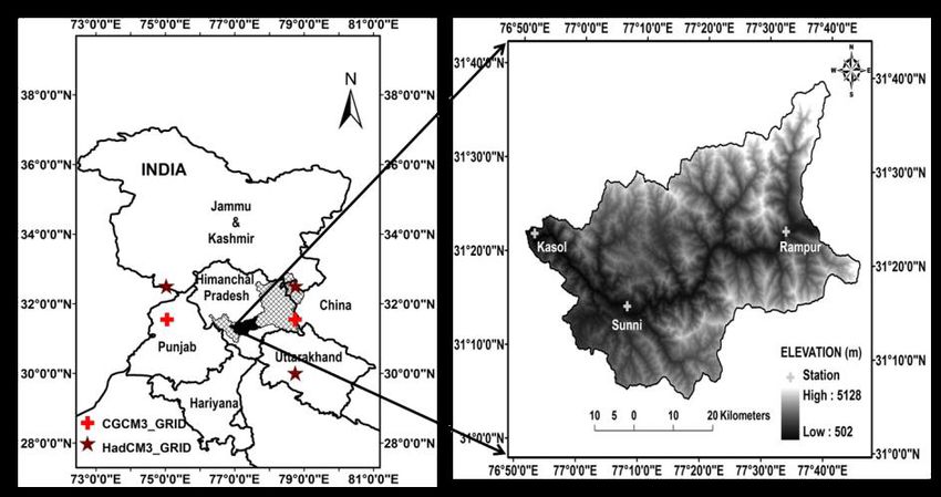
Figure 1: Location map of study area
Figure 2: Location map of study area
international border with China (Tibet). It from Bhakra Beas Management Board (BBMB),
covers a geographical area of 2457km2 lying India for three stations namely, Kasol, Sunni
between 31°05’00”N to 31°39’26”N latitudes and Rampur. These stations have data series
and 76°51’11”E to 77°45’17”E longitudes covering the period 1963-2000 for Kasol and
(Figure 1). 1970-2000 for Sunni and Rampur respectively.
Sutlej river basin is drained by the Sutlej river Figure 1 also shows the location of stations.
which originates from Mansarovar- Rakastal The observed and modelled predictors
lakes near Darma pass in the western Tibet at an are obtained from the National Centre for
elevation of 4,570 m. The basin is characterized Environmental Prediction/ National Centre
by steep slope, dissected topography and high for Atmospheric Research (NCEP/ NCAR)
relief features. The altitude in the basin (study reanalysis (Kalnay et al., 1996) and from
area) ranges in between 502 m to 5128 m. CGCM3 and HadCM3 models respectively.
The slope gradually decreases downstream. The NCEP/NCAR reanalysis data sets have a
The major part of the study area exhibits the grid-spacing of 1.9° latitude × 1.9° longitude
characteristics of warm and temperate climate. whereas CGCM3 and HadCM3 have grid
The mean annual rainfall and temperature is resolution of 3.75° latitude × 3.75° longitude
103cm and 21.23°C respectively. and 2.5° latitude × 3.75° longitude respectively .
Figure 2: Comparing observed and downscaledThe re-gridding
values of the NCEP/NCAR
of precipitation (PCP) for reanalysis
all three
predictors have been performed to conform
3. DATA SETS stations during calibration period fortoCGCM3 and HadCM3
the grid-spacing models
of CGCM3 and HadCM3
The data acquired from various sources are used models. The standardization of predictors
throughout the downscaling procedure. The is carried out before statistical downscaling
climate station precipitation data (predictand) to minimize biases in mean and variance of
21
which is available on daily time step is procured CGCM3 and HadCM3 predictors with respect
Journal of Hydrology and Meteorology, Vol. 9, No. 1 SOHAM-NepalAugust 2015 Dharmaveer Singh, R.D. Gupta & Sanjay K. Jain 5
Table 1: Selection of NCEP/ NCAR predictors using partial correlations and P value statistics
Precipitation (CGCM3 Model) Precipitation (HadCM3 Model)
Station Partial P Partial P
Predictors Predictors
Correlation(r) value Correlation(r) value
p__v 0.027 0.2860 msl -0.114 0.0000
p500 0.076 0.0021 p5_f 0.094 0.0006
p5zh 0.073 0.0032 rhum 0.149 0.0000
Kasol
s850 0.122 0.0000
shum 0.081 0.0010
temp 0.091 0.0002
p_f 0.011 0.5168 p__z -0.059 0.0418
p500 -0.14 0.0000 p__th -0.022 0.3911
p_th -0.080 0.0047 pzh 0.038 0.1925
shum 0.208 0.0000 p5_u -0.036 0.2152
Sunni
p500 -0.086 0.021
p8_th 0.048 0.0973
rhum 0.115 0.0000
temp 0.095 0.0006
msl 0.062 0.0293 p5_v -0.061 0.0149
p_th -0.041 0.1570 temp 0.064 0.0110
p500 -0.153 0.0000
Rampur p8_z 0.120 0.0000
p8zh -0.117 0.0000
s850 0.126 0.0000
temp 0.089 0.0012
to that of NCEP/ NCAR reanalysis data. All the Special Report on Emission Scenarios (SRES)
predictor variables are normalized over baseline A2 and A1B emission scenarios for future run
periods i.e., 1961-1990 periods. for CGCM3 model and A2 and B2 emission
The re-gridded and standardized predictors scenarios for HadCM3 model respectively.
used as the SDSM model input are directly
downloaded from the Data Access Integration 4. METHODOLOGY
(DAI) website (http://loki.qc.ec.gc.ca/DAI/
predictors-e.html) for CGCM3 model and The SDSM 4.2 software, invented by R.L.
Canadian Climate Impacts Scenarios (CCIS) Wilby and C.W. Dawson (Wilby et al., 2002)
website (http://www.cics.uvic.ca/scenarios/ has been used to downscale and generate future
index.cgi) for HadCM3 model. The predictor scenarios of precipitation. It is a windows based
variables are available for period 1961- decision support tool that is based on statistical
2100 for CGCM3 model, 1961-2099 for downscaling method. In this software, the
HadCM3 model and 1961-2001 for NCEP/ multiple liner regression is used to establish
NCAR. The predictors are simulated under A2 empirical relationship between predictors
historical GHG (Greenhouse Gas) and aerosol and predictands whereas downscaled data is
concentration experiment (20C3M) as well as generated stochastically. Therefore, SDSM
Journal of Hydrology and Meteorology, Vol. 9, No. 1 SOHAM-Nepal6 GCMs Derived Projection of Precipitation and Analysis ... August 2015
Table 2: Cross correlation between predictors of NCEP/NCAR (CGCM3model)
Station Predictors
p__v p500 p5zh s850 shum temp
p__v 1 -0.01 0.14 -0.10 0.20 0.14
p500 -0.01 1 -0.54 -0.12 -0.32 -0.33
Kasol p5zh 0.14 0.54 1 0.03 0.04 0.01
s850 -0.10 -0.12 0.03 1 0.87 0.67
shum 0.20 -0.32 0.04 0.87 1 0.70
temp 0.14 -0.33 0.01 0.67 0.70 1
p_f p500 p_th shum
p_f 1 0.10 0.34 0.63
Sunni p_th 0.10 1 0.37 0.29
p500 0.34 0.37 1 0.81
shum 0.63 0.29 0.81 1
msl p_th p500 p8_z p8zh s850 temp
msl 1 -.03 -0.10 -0.10 -0.08 -0.11 0.05
p_th -.03 1 -0.20 -0.58 0.36 -0.26 -0.82
p500 -0.10 -0.20 1 -0.16 0.12 0.82 0.90
Rampur
p8_z -0.10 -0.58 -0.16 1 -0.19 -0.35 -0.28
p8zh -0.08 0.36 0.12 -0.19 1 0.23 0.17
s850 -0.11 -0.26 0.82 -0.35 0.23 1 0.89
temp 0.05 -0.82 0.90 -0.28 0.17 0.89 1
is a hybrid downscaling model comprising a from predictors of NCEP/ NCAR and GCMs.
stochastic weather generator and a regression The performance of the model along with
method (Chen et al., 2010). The development of downscaled results is discussed for future
SDSM tool and its characteristics are discussed periods (2020’s, 2050’s and 2080’s) under
in literature (Wilby et al., 1998, 1999, 2002; various emission scenarios (A2, A1B and B2).
Wilby and Dawson, 2007). The predictor
variables selected for downscaling daily
precipitation used in the study are shown in bold 5.1. Development of SDSM Downscaling
in Table 1. Further, cross correlation between Model
predictors of NCEP/NCAR is also investigated The selected predictors from sets of NCEP/
and it is shown in Table 2 for CGCM3 model. NCAR reanalysis data as given in Table 2 are
A high positive correlation is observed between used to train SDSM 4.2 model. The model
predictors such as shum, s850 and temp. This is calibrated and validated for downscaling
indicates mutual dependency of these predictors precipitation using 20 years (1963-1982 for
with each other. Kasol) data, 16 years (1970-1985 for Sunni and
Rampur) and 18 years (1983-2000 for Kasol),
15 years (1986-2000 for Sunni and Rampur)
5. RESULTS AND DISCUSSIONS data respectively. The statistical parameters
This section describes the development of such as the monthly average percentage
SDSM 4.2 for downscaling of precipitation of explained variance (E) and the monthly
Journal of Hydrology and Meteorology, Vol. 9, No. 1 SOHAM-NepalAugust 2015 Dharmaveer Singh, R.D. Gupta & Sanjay K. Jain 7
Table 3: Performance statistics of SDSM model during calibration period
Precipitation (CGCM3) Precipitation (HadCM3)
Station SE RMSE SE RMSE
E (%) R2 E (%) R2
(mm) (mm) (mm) (mm)
Kasol (1963-82) 11.20 0.082 0.63 3.17 5.00 0.87 0.61 3.43
Sunni (1970-85) 6.40 0.088 0.41 2.13 7.30 0.88 0.37 2.42
Rampur (1970-85) 13.60 0.79 0.46 1.18 8.30 0.081 0.30 1.45
Table 4: Performance statistics of SDSM model during validation period
Precipitation (CGCM3) Precipitation (HadCM3)
Station SE RMSE SE RMSE
E (%) FIGURE CAPTIONS
R2 E (%) R2
(mm) (mm) (mm) (mm)
Kasol (1983-2000) 10.40 0.084 0.58 3.54 4.80 0.87 0.57 3.34
Sunni (1986-2000) 5.90 0.088 0.49 1.89 7.10 0.87 0.34 2.25
Rampur (1986-2000) 13.90 0.79 0.37 1.34 9.90 0.080 0.31 1.46
average standard error (SE) are used to reflect precipitation has been found in between 6.40%
downscaling results of daily precipitation at to 13.60% for CGCM3 model and 5.00(%) to
each site in the basin. To evaluate the efficiency 8.30(%) for HadCM3 model respectively. The
of model performance during calibration period, results gained during validation are listed in
coefficient of determination R2 and Root Mean Table 4.
Square Error (RMSE) statistics are used. A comparison of observed daily precipitation
The results obtained from calibration show with downscaled precipitation has been shown
small values of E (%) and R which reveal
2
in Figure 2 and 3 for calibration and validation
the complexity of downscaling station scale period. The results show that a moderate to poor
precipitation from predictor variables (Table agreement has been observed between observed
3). The monthly average value
Figure of E (%) for
2: Location map ofand downscaled
study area precipitation values.
Figure 2: Comparing observed and downscaled values of precipitation for all three stations during calibration period for
CGCM3 and HadCM3 models
Figure 2: Comparing observed and downscaled values of precipitation (PCP) for all three
Journal of Hydrology and Meteorology, Vol. 9, No. 1 SOHAM-Nepal
stations during calibration period for CGCM3 and HadCM3 models8 GCMs Derived Projection of Precipitation and Analysis ... August 2015
Figure 3: Comparing observed and downscaled values of precipitation (PCP) for all three
stations during validation for CGCM3 and HadCM3 models
Figure 3: Comparing observed and downscaled values of precipitation for all three stations during validation for CGCM3 and
HadCM3 models
Figure 3: Comparing observed and downscaled values of precipitation (PCP) for all three
stations during validation for CGCM3 and HadCM3 models
Figure 4: Box plots results from SDSM based downscaling model for the projected precipitation (CGCM3 model). The horizontal
line in the middle of the box represents median value while darkened square represents mean value of precipitation data
5.2. Spatial and Temporal Patterns of future period is grouped into three time slices;
22
Downscaled Precipitation for Future 2020’s (2011–2040), 2050’s (2041–2070) and
Periods 2080’s (2071–2099) and each corresponds
The calibrated SDSM model is used to to span of 30 year periods respectively. The
downscale and generate future scenarios of22 downscaled precipitation is compared with
precipitation from predictors of CGCM3 baseline precipitation (1970-2000) to observe
(SRES A2 and A1B) and HadCM3 (SRES A2 change in patterns of precipitation.
and B2) models in the study region. The pattern The projected precipitation for the future
of downscaled precipitation is investigated for periods (2020’s, 2050’s and 2080’s) has been
future periods with a box plot. For this study, the shown in Figure 4 for the CGCM3 model.
Journal of Hydrology and Meteorology, Vol. 9, No. 1 SOHAM-Nepalprecipitation (CGCM3 model). The horizontal line in the middle of the box represents median
value while darkened square represents mean value of precipitation data
August 2015 Dharmaveer Singh, R.D. Gupta & Sanjay K. Jain 9
Figure 5: Box plots results from SDSM based downscaling model for the projected precipitation (HadCM3 model).
The horizontal line in the middle of the box represents median value while darkened square represents mean value of
precipitation data
Figure 5: Box plots results from SDSM based downscaling model for the projected
The increase in future precipitation has been 2080’s and 3.77% under A2 and 4.08% under
precipitation
observed at Kasol(HadCM3
and Rampurmodel).
whileThe horizontal B2
decrease linefor
in the middle
2050’s. Forof2020’s,
the boxnorepresents
change in mean
has been found at Sunni for SRES A2 and annual precipitation has been noticed under A2
median value while darkened square
SRES A1B scenarios. An overall increase of represents mean itvalue
whereas of precipitation
is 0.92% under B2datascenario. The
5.67%, 8.52% and 18.25% has been computed poor results obtained during calibration and
in mean annual precipitation in the study area validation suggests that predictors of HadCM3
under A1B scenario during 2020’s, 2050’s and model are not well simulated. Further, these are
2080’s whereas it is 9.21%, 11.23% and 13.91% unable to capture regional climate dynamics
under A2 scenario respectively. The increase in and hence, poorly projected by SDSM model as
projected precipitation is higher for A2 scenario compared to CGCM3 model.
as compared to A1B scenario. The seasonal patterns of projected precipitation
The results obtained from HadCM3 model is have been studied and presented in Table 5 for
shown in Figure 5. The decline in amount of CGCM3 model. The large increase in projected
simulated precipitation has been found at Sunni precipitation has been found at Kasol and
and Rampur whereas increase at Kasol for SRES significant decrease at Sunni during JJA (June,
A2 and SRES B2 scenarios. The net change in July, August) periods. The unexpected results
amount of mean annual precipitation has been have been observed at Rampur. The increase in
computed over study area under SRES A2 and projected precipitation has been shown during
SRES B2 scenarios. The results show increase JJA periods for A1B emission scenario and
in magnitude of precipitation under A2 and B2 decrease for A2 scenario accordingly. The model
scenarios for 2080’s and decrease for 2050’s predicts increase in projected precipitation
respectively. This has been found 5.24% under under SON (September, October, November)
A2 scenario and 4.57% under B2 scenario for periods for all three stations.
23
Journal of Hydrology and Meteorology, Vol. 9, No. 1 SOHAM-Nepal10 GCMs Derived Projection of Precipitation and Analysis ... August 2015
Table 5: Change in projected precipitation during different seasons for CGCM3 model
Change in Precipitation (cm)
Station Season SRES A2 Scenario SRES A1B Scenario
2020’s 2050’s 2080’s 2020’s 2050’s 2080’s
DJF -0.76 -1.95 -2.74 0.41 1.42 2.14
MAM -2.48 -2.79 -2.69 1.25 2.24 2.70
Kasol
JJA 19.15 28.75 49.24 25.90 29.90 41.68
SON 4.13 5.01 12.24 4.78 18.54 7.24
DJF 1.27 0.06 0.38 0.50 2.13 0.50
MAM -3.40 -3.36 -3.39 3.52 3.56 3.43
Sunni
JJA -10.73 -10.46 -8.42 10.07 7.85 9.26
SON 5.37 5.97 6.63 5.33 6.50 7.98
DJF 1.42 0.44 7.26 1.29 1.74 1.22
MAM 3.63 8.92 4.40 0.20 1.20 1.81
Rampur
JJA -0.18 -6.24 -5.83 5.29 4.23 2.17
SON 0.47 2.60 0.41 1.91 2.27 3.60
Table 6: Change in projected precipitation during different seasons for HadCM3 model
Change in Precipitation (cm)
Station Season SRES A2 Scenario SRES B2 Scenario
2020’s 2050’s 2080’s 2020’s 2050’s 2080’s
DJF 19.37 5.11 37.75 18.72 2.39 36.73
MAM 22.13 6.22 9.99 24.04 6.59 8.78
Kasol
JJA -23.99 -6.99 -23.52 -24.52 -5.84 -23.06
SON 1.03 2.48 13.78 0.57 2.13 11.38
DJF -0.023 -2.02 -3.37 -0.65 -1.51 -2.23
MAM 4.78 3.22 0.89 4.55 2.78 2.61
Sunni
JJA -7.98 -6.86 -6.62 -6.57 -5.14 -6.34
SON -1.89 -1.60 -1.87 -1.83 -1.77 -1.80
DJF -3.19 0.20 -2.91 -3.20 -3.01 -3.16
MAM -2.30 -1.94 -2.21 -1.66 -2.19 -2.36
Rampur
JJA -5.02 -4.32 -4.12 -4.85 -5.14 -4.92
SON -2.41 -2.13 -2.12 -2.32 -2.23 -2.20
On contrary, the projected precipitation obtained 6. CONCLUSION
from HadCM3 model (Table 6) show significant In the present paper, a multiple regression
differences in results that are obtained from based statistical downscaling tool popularly
CGCM3 model. The amount of precipitation known as SDSM 4.2 is successfully applied
is reduced significantly during JJA periods at to downscale and generate future scenarios of
Kasol. The decrease in projected precipitation precipitation from predictors of CGCM3 and
has been observed for future periods at Sunni HadCM3 models in a part of North-Western
and Rampur respectively.
Journal of Hydrology and Meteorology, Vol. 9, No. 1 SOHAM-NepalAugust 2015 Dharmaveer Singh, R.D. Gupta & Sanjay K. Jain 11
(N-W) Himalayan region, India. The change REFERENCES
in projected precipitation has been studied for Anandhi, A., Shrinivas, V.V., Nanjundiah,
the time periods; 2020’s, 2050’s and 2080’s for R.S., Kumar, D.N., 2008. Downscaling
SRES A2 and A1B scenarios (CGCM3 model) precipitation to river basin in India for
and for SRES A2 and B2 scenarios respectively. IPCC SRES scenarios using support
The seasonal patterns of precipitation are also vector machine. International Journal of
examined and changes with respect to baseline Climatology 28 (3), 401-420.
period are shown.
Bardossy, A., Bogardi, I., Matyasovszky, I.,
The results of precipitation downscaling using 2005. Fuzzy rule-based downscaling of
SDSM are found to be poor for HadCM3 precipitation. Theoretical and Applied
model as compared to CGCM3 model. The Climatology 82 (1-2), 119–129.
results obtained from CGCM3 model predict an
overall increase in precipitation while decrease Basistha, A., Arya, D.S., Goyal, N.K., 2009.
in precipitation is predicted by HadCM3 model Analysis of historical changes in rainfall
for the future periods in the region. Based on in the Indian Himalayas. International
the analysis of results, CGCM3 model has been Journal of Climatology, 29 (4), 555-572.
found better for simulation of precipitation in Bhutiyani, M. R., Kale, V. S., Pawar, N. J., 2007.
comparison to HadCM3 model. Long-term trends in Maximum, minimum
and mean annual air temperatures across
the northwestern Himalaya during the
APPENDIX: 1 twentieth century. Climatic Change, 85,
Abbreviations used in Table 1 159-177.
Predictors Description Carter, T.R., La Rovere, E.L, Jones, R.N.,
msl Mean sea level pressure Leemans, R., Mearns, L.O., Nakicenovic,
p_f Surface air flow strength
N., Pittock, A.B., Semenov, S.M., Skea
p__v Surface meridional velocity
p__z Surface vorticity
J., 2001. Developing and applying
p_th Surface wind direction scenarios. In J.J. McCarthy, O.F.
pzh Surface divergence Canziani, N.A. Leary, D.J. Dokken &
p5_f 500 hpa airflow strength K.S. White (Eds.), Climate Change 2001:
p5_u 500 hpa zonal velocity Impacts, Adaptation, and Vulnerability.
p5_v 500 hpa meridional velocity
Contribution of Working Group II to
Predictors Description
p500 500 hpa geopotential height the Third Assessment Report of the
p5zh 500hpa divergence Intergovernmental Panel on Climate
p8_z 850 hpa vorticity Change (pp. 145-190), Cambridge
p8_th 850 hpa wind direction University Press, Cambridge.
s850 Relative/Specific humidity at 850 hpa
p8zh 850 hpa divergence Chen, S.-T., Yu, P.-S., Tang, Y.-H., 2010.
rhum Near surface relative humidity Statistical downscaling of daily
shum Surface specific humidity precipitation using support vector
temp Mean temperature at 2 m machines and multivariate analysis.
Journal of Hydrology 385 (1-4), 13-22.
Journal of Hydrology and Meteorology, Vol. 9, No. 1 SOHAM-Nepal12 GCMs Derived Projection of Precipitation and Analysis ... August 2015
Dubrovsky, M., Buchtele, J., Zalud, Z., 2004. Hua, C., Jing, G., Wei, X., Guo, S., Xu, C.-
High-frequency and low frequency Y., 2010. Downscaling GCMs using the
variability in stochastic daily weather Smooth Support Vector Machine Method
generator and its effect on agricultural to predict daily precipitation in the
and hydrologic modelling. Climatic Hanjiang Basin. Advances in Atmospheric
Change 63 (1-3), 145–179. Sciences 27 (2), 274–284.
Farooq, A.B., Khan, A.H., 2004. Climate http://loki.qc.ec.gc.ca/DAI/predictors-e.html
change perspective in Pakistan. In A. [Last accessed date 3/02/2012].
Muhammed & L. Stevenson (Eds.), http://www.cics.uvic.ca/scenarios/index.cgi
Proceedings of Capacity Building APN [Last accessed date 3/02/2012].
Workshop on Global Change Research,
(pp39-46), Islamabad, Pakistan. Jain, S. K., 2012. Sustainable water management
in India considering likely climate and
Fowler, H.J., Kilsby, C.G., O’Connell, P.E., other changes. Current Science 102(2),
2000. A stochastic rainfall model 117-188.
for the assessment of regional water
Jones, R.G., Murphy, J.M., Noguer, M., 1995.
resource systems under changed climatic
Simulation of climate change over
conditions. Hydrology and Earth System
Europe using a nested regional climate
Sciences 4 (2), 261–280.
model. I. Assessment of control climate,
Ghosh, S., 2010. SVM-PGSL coupled approach including sensitivity to location of lateral
for statistical downscaling to predict boundaries. Quarterly Journal of the
rainfall from GCM output. Journal of Royal Meteorological Society, 121(526),
Geophysical Research 115, D22102. 1413–1450
Ghosh, S., Mishra, C., 2010. Assessing Kalnay, E., Kanamitsu, M., Kistler, R., Collins,
hydrological impacts of climate change: W., Deaven, D., Gandin, L., Iredell, M.,
modeling techniques and challenges. The Saha, S., White, G., Woollen, J., Zhu,
Open Hydrology Journal 4, 115-121. Y., Chelliah, M., Ebisuzaki, W., Higgins,
W., Janowiak, J., Mo, K.C.,, Ropelewski,
Giorgi, F., 1990. Simulation of regional climate
C., Wang, J., Leetmaa, A., Reynolds,
using a limited area model nested in a
R., Jenne, R., Joseph, D., 1996. The
general circulation model. Journal of
NCEP/NCAR 40-year reanalysis project.
Climate 3(9), 941–963.
Bulletin of the American Meteorological
Gosain, A.K., Rao, S., Arora, A., 2011. Climate Society, 77(3), 437–471.
change impact assessment of water
Kim, J. W., Chang, J. T., Baker, N. L.,
resources of India. Current Science,
Wilks, D. S., Gates, W. L., 1984. The
101(3), 356-371.
statistical problem of climate inversion:
Hewitson, B. C., Crane, R.G., 1996. Climate Determination of the relationship between
downscaling: techniques and application. local and large-scale climate. Monthly
Climate Research 7 (2), 85–95. Weather Review, 112 (10), 2069–2077.
Journal of Hydrology and Meteorology, Vol. 9, No. 1 SOHAM-NepalAugust 2015 Dharmaveer Singh, R.D. Gupta & Sanjay K. Jain 13
Kumar, V., Jain, S.K., 2010. Trends in rainfall Raghavan, S.V., Vu, M.T., Liong, S.Y., 2012.
amount and number of rainy days in river Assessment of future stream flow over
basins of India (1951–2004). Hydrology the Sesan catchment of the Lower
Research, 42(4), 290–306. Mekong Basin in Vietnam. Hydrological
Process, 26 (4), 3661-3668, doi: 10.1002/
Kumar, V., Singh, P., Jain S.K., 2005,
hyp.8452
(April). Rainfall trends over Himachal
Pradesh, Western Himalaya, India. In Raje, D., Mujumdar, P. P, 2011. A comparison
G.N., Mathur, A.S., Chawla, & R.L., of three methods for downscaling daily
Chauhan (Eds),Conference Proceedings, precipitation in the Punjab region.
Development of Hydro Power Projects Hydrological Process, 25(23), 3575-
– A Prospective Challenge (II-63-II-71), 3589.
organized by CBIP & HPSEB, Shimla, Rupa Kumar, K. R., Sahai, A. K., Krishna, K.
New Delhi, India. K., Patwardhan, S. K., Mishra, P. K.,
Kilsby, C.G., Jones, P.D., Burton, A., Ford, Revadkar, J. V., Kamala, K., Pant, G. B.,
A.C., Fowler, H.J., Harpham, C., James, 2006. High resolution climate change
P., Smith, A., Wilby, R.L., 2007. A daily scenario for India for the 21st century.
weather generator for use in climate Current Science 90 (3), 334–345.
change studies. Environmental Modelling Shrestha, A.B., Wake, C.P., Dibb, J.E.,
and Software, 22(12), 1705–1719. Mayyewski, P.A., 2000. Precipitation
fluctuations in the Nepal Himalaya and
Lapp, S., Sauchyn, D., Toth, B., 2009.
its vicinity and relationship with some
Constructing scenarios of future climate
large-scale climatology parameters.
and water supply for the SSRB: Use and
International Journal of Climatology
limitations for vulnerability assessment.
20(3), 317–327.
Prairie Forum (Guest Issue), 34(1), 153-
180. Tripathi, S., Srinivas, V.V., Nanjundiah, R.S.,
2006. Downscaling of precipitation for
Mason, S.J., 2004. Simulating Climate over climate change scenarios: a support vector
Western North America Using Stochastic machine approach. Journal of Hydrology
Weather Generators. Climatic Change, 330 (3–4), 621–640.
62(1-3), 155–187.
von Storch, H., Langenberg, H., Feser, F.,
Pant, G.B., Rupa, Kumar, R.R., Borgaonkar, 2000. A spectral nudging technique
H.P., 1999. Climate and its long-term for dynamical downscaling purposes.
variability over the western Himalaya Monthly Weather Review 128 (10), 3664–
during the past two centuries. In 3673.
S.K., Dash, & J., Bahadur, (Eds). The Wilby, R.L., Hassan, H., Hanaki, K.,
Himalayan Environment (pp. 171- 1998. Statistical downscaling of
184), New Age International (P) Ltd., hydrometeorological variables using
Publishers: New Delhi, India. general circulation model output. Journal
of Hydrology 205 (1-2), 1-19.
Journal of Hydrology and Meteorology, Vol. 9, No. 1 SOHAM-Nepal14 GCMs Derived Projection of Precipitation and Analysis ... August 2015
Wilby, R.L., Hay, L.E., Leavesly, G.H., 1999. A Wilby, R. L., Wigley, T. M. L., 1997. Downscaling
comparison of downscaled and raw GCM general circulation model output: a review
output: implications for climate change of methods and limitations. Progress in
scenarios in the San Juan River Basin, Physical Geography 21(4), 530–548.
Colorado. Journal of Hydrology, 225 (1- Xu, Y.C., 1999. From GCMs to river flow:
2), 67–91. a review of downscaling methods and
Wilby, R.L., Dawson, C.W., Barrow, E.M., hydrologic modelling approaches.
2002. SDSM - a decision support tool for Progress in Physical Geography, 23(2),
the assessment of regional climate change 229–249.
impacts. Environmental Modelling & Xu, Z., Gong, T., Liu, C., 2008. Decadal
Software, 17(2), 147-159. trends of climate in the Tibetan Plateau
Wilby, R.L., Dawson, C.W., 2007. SDSM User – regional temperature and precipitation.
Manual- A Decision Support Tool for the Hydrological Processes, 22 (16), 3056–
Assessment of Regional Climate Change 3065.
Impacts. Retrieved from https://copublic. Zhao L, Ping C L, Yang D Q et al., 2004. Change
lboro.ac.uk/cocwd/SDSM/main.html of climate and seasonally frozen ground
[Last accessed date 17.11.2011. over the past 30 years in Qinghai-Tibetan
plateau, China’. Global and Planetary
Change, 43, 19–31.
Journal of Hydrology and Meteorology, Vol. 9, No. 1 SOHAM-NepalYou can also read