3D free-form object recognition in range images using local surface patches
←
→
Page content transcription
If your browser does not render page correctly, please read the page content below
Pattern Recognition Letters 28 (2007) 1252–1262
                                                                                                                       www.elsevier.com/locate/patrec

                        3D free-form object recognition in range images
                                   using local surface patches
                                                        Hui Chen, Bir Bhanu                 *

                            Center for Research in Intelligent Systems, University of California, Riverside, CA 92521, USA

                                          Received 20 April 2006; received in revised form 25 January 2007
                                                        Available online 28 February 2007

                                                        Communicated by G. Sanniti di Baja

Abstract

    This paper introduces an integrated local surface descriptor for surface representation and 3D object recognition. A local surface
descriptor is characterized by its centroid, its local surface type and a 2D histogram. The 2D histogram shows the frequency of occur-
rence of shape index values vs. the angles between the normal of reference feature point and that of its neighbors. Instead of calculating
local surface descriptors for all the 3D surface points, they are calculated only for feature points that are in areas with large shape var-
iation. In order to speed up the retrieval of surface descriptors and to deal with a large set of objects, the local surface patches of models
are indexed into a hash table. Given a set of test local surface patches, votes are cast for models containing similar surface descriptors.
Based on potential corresponding local surface patches candidate models are hypothesized. Verification is performed by running the Iter-
ative Closest Point (ICP) algorithm to align models with the test data for the most likely models occurring in a scene. Experimental
results with real range data are presented to demonstrate and compare the effectiveness and efficiency of the proposed approach with
the spin image and the spherical spin image representations.
 2007 Elsevier B.V. All rights reserved.

Keywords: 3D object recognition; Local surface patch; Model indexing; Free-form surface registration; Range images

1. Introduction                                                              sor can provide geometric information about objects which
                                                                             is less sensitive to the above imaging problems. As a result,
   3D object recognition, an important research field of                      the design of a recognition system using 3D range data has
computer vision and pattern recognition, involves two                        received significant attention over the years.
key tasks: object detection and object recognition. Object                       In 3D object recognition, the key problems are how to
detection determines if a potential object is present in a                   represent free-form surfaces effectively and how to match
scene and its location; object recognition determines the                    the surfaces using the selected representation. In the
object ID and its pose (Suetens et al., 1992). Researchers                   early years of 3D computer vision (Besl and Jain, 1985;
have done an extensive research on recognizing objects                       Chin and Dyer, 1986), the representation schemes included
from 2D intensity images. It has been challenging to design                  Wire-Frame, Constructive Solid Geometry (CSG),
a system based on 2D intensity images which can handle                       Extended Gaussian Image (EGI), Generalized Cylinders
problems associated with changing 3D pose, lighting and                      and planar faces (Bhanu, 1984; Faugeras and Hebert,
shadows effectively. The 3D data collected by a range sen-                    1986). Early work mainly dealt with the polyhedral objects.
                                                                             It segmented curved surfaces into planar surfaces. How-
 *
   Corresponding author. Tel.: +1 9097873954; fax: +1 9097873188.
                                                                             ever, the planar patch is not the most suitable representa-
   E-mail addresses: hchen@vislab.ucr.edu (H. Chen), bhanu@vislab.           tion for free-from surfaces and researchers have used a
ucr.edu (B. Bhanu).                                                          number of representations, including B-Splines (Bhanu

0167-8655/$ - see front matter  2007 Elsevier B.V. All rights reserved.
doi:10.1016/j.patrec.2007.02.009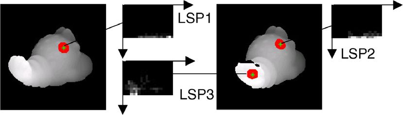
H. Chen, B. Bhanu / Pattern Recognition Letters 28 (2007) 1252–1262                         1253

and Ho, 1987), surface curvatures, superquadrics (Solina             table for fast retrieval and matching. Hypotheses are gener-
and Bajcsy, 1990) and deformable models to recognize                 ated by casting votes to the hash table and false hypotheses
free-form objects in range images (Campbell and Flynn,               are removed by estimating rigid transformations. Chua and
2001). Other recent surface representations include the              Jarvis (1997) used the point signature representation, which
splash representation (Stein and Medioni, 1992), the point           describes the structural neighborhood of a point, to repre-
signature (Chua and Jarvis, 1997), the spin image (Johnson           sent 3D free-form objects. Point signature is 1D signed dis-
and Hebert, 1999), the surface point signature (Yamany               tance profile with respect to the rotation angle defined by
and Farag, 1999), the harmonic shape image (Zhang and                the angle between the normal vector of the point on the
Hebert, 1999), the spherical spin image (Correa and Shap-            curve and the reference vector. Recognition is performed
iro, 2001), the 3D point’s ‘‘fingerprint’’ (Sun and Abidi,            by matching the signatures of points on the scene surfaces
2001) and the 3D shape contexts and harmonic shape con-              to those of points on the model surfaces. The maximum
texts (Frome et al., 2004).                                          and minimum values of the signatures are used as indexes
   In this paper, we introduce an integrated local surface           to a 2D table for fast retrieval and matching.
descriptor for 3D object representation. We calculate the               Johnson and Hebert (1999) presented the spin image (SI)
local surface descriptors only for the feature points which          representation for range images. Given an oriented point on
are in the areas with large shape variation measured by              a 3D surface, its shape is described by two parameters: dis-
shape index (Dorai and Jain, 1997). Our approach starts              tance to the tangent plane of the oriented point from its
from extracting feature points in range images, then defines          neighbors and the distance to the normal vector of the ori-
the local surface patch at each of the feature points (Chen          ented point. The approach involved three steps: generating
and Bhanu, 2004). Next we calculate local surface proper-            a spin image, finding corresponding points and verifying
ties of a patch. These properties are 2D histogram, surface          hypotheses. First, spin images are calculated at every vertex
type and the centroid. The 2D histogram consists of shape            of the model surfaces. Then the corresponding point pair is
indexes and angles between the normal of the feature point           found by computing the correlation coefficient of two spin
and that of its neighbors. The surface of a patch is classified       images centered at those two points. Next the corresponding
into different types based on the mean and Gaussian curva-            pairs are filtered by using geometric constraint. Finally, a
tures of the feature point. For every local surface patch, we        rigid transformation is computed and a modified Iterative
compute the mean and standard deviation of shape indexes             Closest Point (ICP) algorithm is used for verification. In
and use them as indexes to a hash table. By comparing                order to speed up the matching process, principal component
local surface patches for a model and a test image, and              analysis (PCA) is used to compress spin images. Correa and
casting votes for the models containing similar surface              Shapiro (2001) proposed the spherical spin image (SSI)
descriptors, the potential corresponding local surface               which maps the spin image to points onto a unit sphere. Cor-
patches and candidate models are hypothesized. Finally,              responding points are found by computing the angle between
we estimate the rigid transformation based on the corre-             two SSIs. Yamany and Farag (1999) introduced the surface
sponding local surface patches and calculate the match               signature representation which is a 2D histogram, where one
quality between the hypothesized model and test image.               parameter is the distance between the center point and every
   The rest of the paper is organized as follows. Section 2          surface point and the other one is the angle between the nor-
introduce the related work and contributions. Section 3              mal of the center point and every surface point. Signature
presents our approach to represent the free-form surfaces            matching is done by template matching.
and matching the surface patches. Section 4 gives the                   Zhang and Hebert (1999) introduced harmonic shape
experimental results to demonstrate the effectiveness and             images (HSI) which are 2D representation of 3D surface
efficiency of the proposed approach and compares them                  patches. HSIs are unique and they preserve the shape and
with the spin image and spherical spin image representa-             continuity of the underlying surfaces. Surface matching is
tions. Section 5 provides the conclusions.                           simplified to matching harmonic shape images. Sun and
                                                                     Abidi (2001) introduced 3D point’s ‘‘fingerprint’’ represen-
2. Related work and contributions                                    tation which is a set of 2D contours formed by the projec-
                                                                     tion of geodesic circles onto the tangent plane. Each point’s
2.1. Related work                                                    fingerprint carried information of the normal variation
                                                                     along geodesic circles. Corresponding points are found by
   Stein and Medioni (1992) used two different types of               comparing the fingerprints of points. Frome et al. (2004)
primitives, 3D curves and splashes, for representation               introduced two regional shape descriptors, 3D shape con-
and matching. 3D curves are defined from edges and they               texts and harmonic shape contexts, for recognizing 3D
correspond to the discontinuity in depth and orientation.            objects. The 3D shape context is the straightforward exten-
For smooth areas, splash is defined by surface normals                sion of 2D shape contexts (Belongie et al., 2002) and the
along contours of different radii. Both of the primitives             harmonic shape context is obtained by applying the har-
can be encoded by a set of 3D super-segments, which are              monic transformation to the 3D shape context. Objects
described by the curvature and torsion angles of a super-            are recognized by comparing the distance between the rep-
segment. The 3D super-segments are indexed into a hash               resentative descriptors.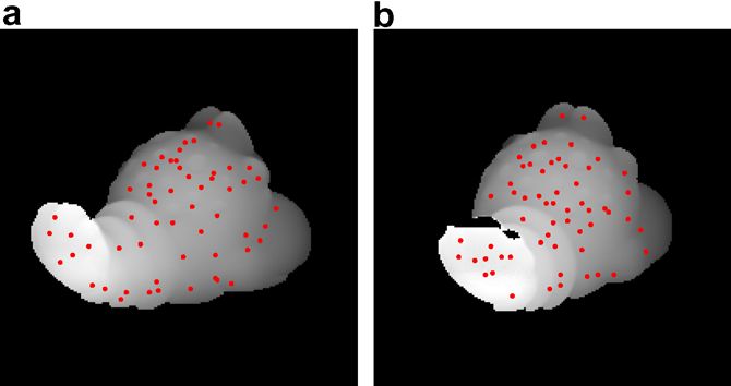
1254                                    H. Chen, B. Bhanu / Pattern Recognition Letters 28 (2007) 1252–1262

2.2. Contributions                                                         Gaussian and mean curvatures and principal curvatures
                                                                           (Bhanu and Chen, 2003; Flynn and Jain, 1989). We move
   The contributions of this paper are: (a) A new local sur-               the local window around and repeat the same procedure
face descriptor, called LSP representation, is proposed for                to compute the shape index value for other points.
surface representation and 3D object recognition. (b) The                     Shape index (Si), a quantitative measure of the shape of
LSP representation is compared to the spin image (Johnson                  a surface at a point p, is defined by (1) where k1 and k2 are
and Hebert, 1999) and spherical spin image (Correa and                     maximum and minimum principal curvatures, respectively
Shapiro, 2001) representations for its effectiveness and effi-
ciency. (c) Experimental results on a dataset of 20 objects                            1 1      k 1 ðpÞ þ k 2 ðpÞ
                                                                           S i ðpÞ ¼     tan1                   :                                ð1Þ
(with/without occlusions) are presented to verify and com-                             2 p      k 1 ðpÞ  k 2 ðpÞ
pare the effectiveness of the proposed approach.
                                                                              With this definition, all shapes are mapped into the
                                                                           interval [0, 1] (Dorai and Jain, 1997). Larger shape index
3. Technical approach                                                      values represent convex surfaces and smaller shape index
                                                                           values represent concave surfaces (Koenderink and Doorn,
  The proposed approach is described in Table 1. It has                    1992). Fig. 1 shows the range image of an object and its
two stages: offline model building and online recognition.                   shape index image. In Fig. 1a, the darker pixels are away
                                                                           from the camera while the lighter ones are closer. In
3.1. Feature points extraction                                             Fig. 1b, the brighter points denote large shape index values
                                                                           which correspond to ridge and dome surfaces while the
   In our approach, feature points are defined in areas with                darker pixels denote small shape index values which corre-
large shape variation measured by shape index calculated                   spond to valley and cup surfaces. From Fig. 1, we can see
from principal curvatures. In order to estimate the curva-                 that shape index values can capture the characteristics of
ture of a point on the surface, we fit a quadratic surface                  the shape of objects, which suggests that shape index can
f(x, y) = ax2 + by2 + cxy + dx + ey + f to a local window                  be used for feature point extraction. In other words, the
centered at this point and use the least square method to                  center point is marked as a feature point if its shape index
estimate the parameters of the quadratic surface, and then                 Si satisfies Eq. (2) within a w · w window
use differential geometry to calculate the surface normal,
                                                                           S i ¼ max of shape indexes and S i P ð1 þ aÞ  l;
Table 1
                                                                           or S i ¼ min of shape indexes and S i 6 ð1  bÞ  l;
Algorithms for recognizing 3D objects in a range image                                 1 XM

(a) For each model object
                                                                           where l ¼         S i ðjÞ 0 6 a; b 6 1:                                 ð2Þ
                                                                                      M j¼1
{
    Extract feature points (Section 3.1);
    Compute the LSP descriptors for the feature points (Section 3.2);      In Eq. (2) a, b parameters control the selection of feature
    for each LSP                                                           points and M is the number of points in the local window.
    {                                                                      The results of feature extraction are shown in Fig. 2, where
        Compute (l, r) of the shape index values and use them to index     the feature points are marked by red dots. From Fig. 2, we
        a hash table;
        Save the model ID and LSP into the corresponding entry in the
                                                                           can clearly see that some feature points corresponding to
        hash table; (Section 3.3)                                          the same physical area appear in both images.
    }
}
(b) Given a test object
{
    Extract feature points (Section 3.1);
    Compute the LSP descriptors for the feature points (Section 3.2);
    for each LSP
    {
        Compute (l, r) of the shape index values and use them to index
        a hash table;
        Cast votes to the model objects which have a similar LSP (Sec-
        tion 3.4.1);
    }
    Find the candidate models with the highest votes (Section 3.4.2);
    Group the corresponding LSPs for the candidate models (Section
    3.4.2);
    Use the ICP algorithm to verify the top hypotheses (Section 3.5);
                                                                           Fig. 1. (a) A range image and (b) its shape index image. In (a), the darker
}
                                                                           pixels are away from the camera and the lighter ones are closer. In (b), the
(a) Algorithm for constructing the model database (offline stage).           darker pixels correspond to concave surfaces and the lighter ones
(b) Algorithm for recognizing a test object (online stage).                correspond to convex surfaces.
H. Chen, B. Bhanu / Pattern Recognition Letters 28 (2007) 1252–1262 1255
the cosine of the angle (cos h) between the surface normal
vectors at P and one of its neighbors in N. It is equal to
the dot product of the two vectors and it is in the range
[1, 1]. In (4), bfc is the floor operator which rounds f down
to the nearest integer; (hx, vy) are the indexes along the hor-
izontal and vertical axes respectively and (bx, by) are the bin
intervals along the horizontal and vertical axes, respec-
tively. In order to reduce the effect of the noise, we use
bilinear interpolation when we calculate the 2D histogram.
One example of the 2D histogram is shown as a gray scale
image in Fig. 3; the brighter areas in the image correspond
Fig. 2. Feature points location (Æ) in two range images, shown as gray
to bins with more points falling into them. Note that in the
scale images, of the same object taken at different viewpoints. 2D histogram in Fig. 3 some of the areas are black since no
points are falling into those bins
3.2. Local surface patches (LSP) Si cos h þ 1
hx ¼ ; vy ¼ : ð4Þ
bh by
We define a ‘‘local surface patch’’ as the region consist-
The surface type Tp of a LSP is obtained based on the
ing of a feature point P and its neighbors N. The LSP rep- Gaussian and mean curvatures of the feature point using
resentation includes its surface type Tp, centroid of the Eq. (5) (Besl and Jain, 1988; Bhanu and Nuttall, 1989)
patch and a histogram of shape index values vs. dot prod- where H are mean curvatures and K are Gaussian curva-
uct of the surface normal at the feature point P and its tures. There are eight surface types determined by the signs
neighbors N. A local surface patch is shown in Fig. 3. of Gaussian and mean curvatures given in Table 2. The
The neighbors N satisfy the following conditions: centroid of local surface patches is also calculated for the
N ¼ fpixels N ; kN P k 6 1 g and acosðnp nn Þ < A; ð3Þ computation of the rigid transformation. Note that a fea-
ture point and the centroid of a patch may not coincide.
where • denotes the dot product between the surface nor- In summary, every local surface patch is described by a
mal vectors np and nn at the feature point P and at a neigh- 2D histogram, surface type Tp and the centroid. The 2D
boring point of N, respectively. The acos denotes the histogram and surface type are used for comparison of
inverse cosine function. The two parameters 1 and A are LSPs and the centroid is used for grouping corresponding
important since they determine the descriptiveness of the LSPs and computing the rigid transformation, which will
local surface patch representation. For every point Ni be explained in the following sections. The local surface
belonging to N, we compute its shape index value and patch encodes the geometric information of a local surface
the angle h between the surface normals at the feature point T p ¼ 1 þ 3ð1 þ sgnH ðH ÞÞ þ ð1 sgnK ðKÞÞ;
P and Ni. Then we form a 2D histogram by accumulating 8
points in particular bins along the two axes based on Eq. < þ1 if X > x ;
>
(4) which relates the shape index value and the angle to sgnx ðX Þ ¼ 0 if jX j 6 x ; ð5Þ
>
:
the 2D histogram bin (hx, vy). One axis of this histogram 1 if X < x :
is the shape index which is in the range [0, 1]; the other is
3.3. Hash table building
Local surface patch
Considering the uncertainty of location of a feature
point, we also calculate descriptors of local surface patches
2D histogram
Shape index Table 2
Cosθ
Surface type Tp based on the signs of mean curvature (H) and Gaussian
curvature (K)
Mean curvature H Gaussian curvature K
SurfaceType Tp = 1 K>0 K=0 K1256 H. Chen, B. Bhanu / Pattern Recognition Letters 28 (2007) 1252–1262
Mid Surface Type Histogram Mid Surface Type Histogram
σ, & Centroid & Centroid
std
Mid Surface Type Histogram Mid Surface Type Histogram
& Centroid & Centroid
μ, mean
Accumulator of votes
Model object
Fig. 4. Structure of the hash table. Every entry in the hash table has a linked list which saves information about the model LSPs and the accumulator
records the number of votes that each model receives.
for neighbors of a feature point P. To speed up the retrieval where Q and V are the two normalized histograms and qi
of local surface P patches, for each LSP we compute the and vi are the numbers in the ith bin of the histogram for
mean l ¼ L1 Ll¼1 S i ðpl Þ and standard deviation ðr2 ¼ Q and V, respectively.
1
PL 2 From (6), we know the dissimilarity is between 0 and 2.
L1 l¼1 ðS i ðp l Þ lÞ Þ of the shape index values in N where
If the two histograms are exactly the same, the dissimilarity
L is the number of points on the LSP under consideration
will be zero. If the two histograms do not overlap with each
and pl is the lth point on the LSP. Then we use them to
other, it will achieve the maximum value 2.
index a hash table and insert into the corresponding hash
Fig. 5 and Table 3 show an experimental validation that
bin the information about the model LSPs. Therefore,
the local surface patch is view-invariant and has the dis-
the model local surface descriptors are saved into the hash
criminative power to distinguish shapes. We do experi-
table. For each model object, we repeat the same process to
ments under two cases: (1) a local surface patch (LSP1)
build the model database. The structure of the hash table is
generated for an object is compared to another local sur-
explained in Fig. 4, where every bin in the hash table has an
face patch (LSP2) corresponding to the same physical area
associated linked list which saves the information of the
of the same object imaged at a different viewpoint; a low
model surface descriptors in terms of model ID, 2D histo-
dissimilarity (v2(LSP1, LSP2) = 0.24) is found between
gram, surface type and the centroid; and the accumulator
LSP1 and LSP2 and they have the same surface type. (2)
keeps track of the number of votes that each model
LSP1 is compared to LSP3 which lies in a different area
obtains.
of the same object; the dissimilarity (v2(LSP1, LSP3) =
1.91) is high even though they happen to have the same sur-
3.4. Recognition
face type. The experimental results suggest that the local
surface patch representation provides distinguishable fea-
3.4.1. Comparing local surface patches
tures and it can be used for distinguishing objects. Table
Given a test range image, we extract feature points and
3 lists the comparison of LSPs. We observe that the two
get local surface patches. Then we calculate the mean and
similar local surface patches (LSP1 and LSP2) have close
stand deviation of the shape index values in N for each
mean and standard deviation of the shape index values
LSP, and cast votes to the hash table if the histogram dis-
(compared to other combinations); they can be used for
similarity between a test LSP and a model LSP falls within
fast retrieval of local surface patches.
a preset threshold 2 and the surface type is the same.
Since a histogram can be thought of as an approximation
Table 3
of a probability density function, it is natural to use the Comparison results for three local surface patches shown in Fig. 5
v2 divergence function (6) to measure the dissimilarity
Mean Std. Surface type v2 divergence
(Schiele and Crowley, 2000)
LSP1 0.672 0.043 9 v2(LSP1, LSP2) = 0.24
X ðq vi Þ2 LSP2 0.669 0.038 9 v2(LSP1, LSP3) = 1.91
i
v2 ðQ; V Þ ¼ ; ð6Þ
i þ vi
q LSP3 0.274 0.019 9
i
Fig. 5. Demonstration of discriminatory power of local surface patches. The 2D histograms of three LSPs are displayed as gray scale images. The axes for
the LSP image are the same as shown in Fig. 3. Note that LSP1 and LSP2 are visually similar and LSP1 and LSP3 are visually different.H. Chen, B. Bhanu / Pattern Recognition Letters 28 (2007) 1252–1262 1257
3.4.2. Grouping corresponding pairs of local surface patch
After voting by all the LSPs contained in a test object,
we histogram all hash table entries and get models which
receive the highest votes. From the casted votes, we know
not only the models which get higher votes, but also the
potential corresponding local surface patch pairs. Note
that a hash table entry may have multiple items, we choose
the local surface patch with the minimum dissimilarity and
the same surface type as the possible corresponding patch.
We filter the possible corresponding pairs based on the geo-
metric constraint,
d C1 ;C2 ¼ jd S 1 ;S 2 d M 1 ;M 2 j < 3 ; ð7Þ
where d S 1 ;S 2 and d M 1 ;M 2 are the Euclidean distances between
centroids of the two surface patches. The constraint (7)
guarantees that the distances d S 1 ;S 2 and d M 1 ;M 2 are consis-
tent. For two correspondences C1 = {S1, M1} and
C2 = {S2, M2} where S is the test surface patch and M is
the model surface patch, they should satisfy (7) if they
are consistent corresponding pairs. Therefore, we use the
simple geometric constraint (7) to partition the potential
corresponding pairs into different groups. The larger the
group is, the more likely it contains the true corresponding
pairs.
Given a list of corresponding pairs L = {C1, C2, . . . , Cn},
the grouping procedure for every pair in the list is as fol-
lows: (a) Use each pair as a group of an initial matched
pair. (b) For every group, add other pairs to it if they sat-
isfy (7). (c) Repeat the same procedure for every group. (d)
Select the group which has the largest size.
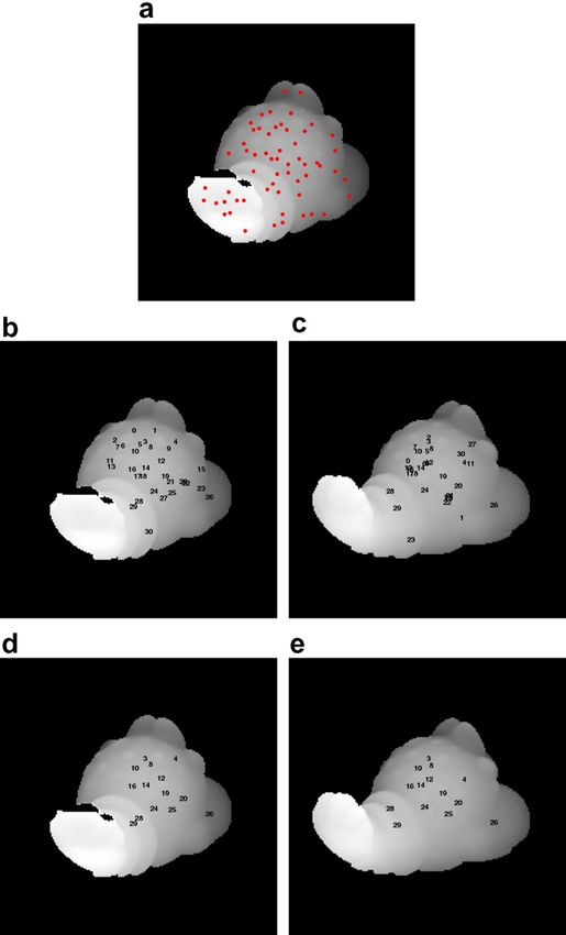
Fig. 6 shows one example of partitioning corresponding
pairs into groups. Fig. 6a shows the feature point extrac-
tion results for a test object. Comparing the local surface
patches with the LSPs on the model objects and querying
the hash table, the initial corresponding LSP pairs are Fig. 6. An example of corresponding LSPs. (a) Feature points marked as
shown in Fig. 6b and c, in which every pair is represented dots on the test object. (b) Test object with matched LSPs after hashing.
by the same number superimposed on the test and model (c) A model object with matched LSPs after hashing. (d) Test object in (b)
with matched LSPs after applying the geometric constraint (7). (e) The
object images. We observe that both of true and false model object in (c) with matched LSPs after applying the geometric
corresponding pairs are found. After applying the geomet- constraint (7).
ric constraint (7), the filtered largest group is shown in
Fig. 6d and e, in which the pairs satisfying the constraint
(7) are put into one group. We observe that true correspon- the quaternion representation (Horn, 1987). Given the esti-
dences between the model and the test objects are obtained mate of initial rigid transformation, the Iterative Closest
by comparing local surface patches, casting votes to the Point (ICP) algorithm (Besl and Mckay, 1992) determines
hash table and using the simple geometric constraint. if the match is good and to find a refined alignment
between them. If the test object is really an instance of
3.5. Verification the model object, the ICP algorithm will result in a good
registration and a large number of corresponding surface
Given the v corresponding LSPs between a model-test points between the model-test pair will be found. Since
pair, the initial rigid transformation, which brings the ICP algorithm requires that the test data set be a subset
model and test objects into coarse alignment, can be esti- of the model set, we use the modified ICP algorithm pro-
mated by minimizing
Pv the sum of the squares of alignment posed by Zhang, 1994 to remove outliers based on the dis-
2
errors R ¼ 1v l¼1 jU l R M l T j with respect to the tance distribution.
rotation matrix R and the translation vector T where Ul Starting with the initial transformation obtained from
and Ml are the centroids of a corresponding LSP pair the coarse alignment, the modified ICP algorithm is run
between the test LSP Ul and the model LSP Ml. The rota- to refine the transformation by minimizing the distance
tion matrix and translation vector are computed by using between the randomly selected points of the model object1258 H. Chen, B. Bhanu / Pattern Recognition Letters 28 (2007) 1252–1262
and their closest points of the test object. For each object in from the UND dataset (UND, 2002). We have used all
the model database, the points are randomly selected three datasets (OSU, UCR, UND) to evaluate the robust-
and the modified ICP algorithm is applied to those points. ness and rotation invariance of the LSP representation (see
The same procedure with random selection of points is Section 4.4).
repeated 15 times and the rigid transformation with the
minimum root mean square (RMS) error is chosen. The 4.2. Single-object scenes
object at the top of the sorted list of model objects with
the minimum RMS error is declared as the recognized These test cases show the effectiveness of the voting
object. In the modified ICP algorithm, the speed bottleneck scheme and the discriminating power of LSPs in the
is the nearest neighbor search. Therefore, the kd-tree struc- hypothesis generation. For a given test object, feature
ture is used in the implementation. points are extracted and the properties of LSPs are calcu-
lated. Then LSPs are indexed into the database of model
4. Experimental results LSPs. For each model indexed, its vote is increased by
one. We show the voting results (shown as a percentage
4.1. Data and parameters of the number of LSPs in the scene which received votes)
for the 20 objects in Fig. 8. Note that in some cases the
We use real range data collected by Ohio State Univer- numbers shown are larger than 100 since some LSPs may
sity (OSU, 1999). There are 20 objects in our database and receive more than one vote. We observe that most of the
the range image of the model objects are shown in Fig. 7. highest votes go to the correct models. For every test
The parameters of our approach are 1 = 6.5 mm, A = p/ object, we perform the verification for the top three models
3, 2 = 0.75, 3 = 9.4 mm, a = 0.35, b = 0.2, and H = K = which obtained the highest votes. The verification results
0.003. For the LSP computation, the number of bins in the are listed in Table 4, which shows the candidate model
shape index axis is 17 and the number of bins in the other ID and the corresponding RMS registration error. From
axis is 34. The total number of LSPs calculated for the Table 4, we observe that all the test objects are correctly
model objects is about 34,000. The average size of local sur- recognized. In order to examine the recognition results
face patch is 230 pixels and the average number of pixels on visually, we display the model object and test object in
an object is 11,956. We apply our approach to the single- the same image before and after the alignment for four
object and the two-object scenes. The model objects and examples. The images in Fig. 9a show test objects and their
scene objects are captured at two different viewpoints. All corresponding model objects before alignment; the images
the 20 model-test pairs are 20 apart except the pairs of in Fig. 9b show test objects and the correctly recognized
object 3, 14 and 19 that are 36 apart. model objects after alignment. We observe that each model
We have also used a large UCR ear database (pose var- object is well aligned with the corresponding test object and
iation ±35) of 155 subjects with 902 images (UCR, 2006). the test cases with large pose variations are correctly han-
In addition, we have used images with large pose variation dled. Since the proposed LSP representation consists of
Fig. 7. The range images of objects in the model database. The object IDs (0–19) are labeled from left to right and top to bottom.H. Chen, B. Bhanu / Pattern Recognition Letters 28 (2007) 1252–1262 1259
0 1 2 3 4 5 6 7 8 9 10 11 12 13 14 15 16 17 18 19
0 69 16 69 27 36 11 40 7 33 24 49 60 33 7 20 16 4 0 51 49
1 51 116 75 44 46 30 42 40 104 53 100 118 79 32 38 2 67 14 65 79
2 63 56 146 54 61 8 76 41 78 54 82 76 49 45 39 8 52 2 53 63
3 21 21 60 76 44 7 44 39 55 10 55 63 71 31 18 10 31 0 10 50
4 35 44 30 25 69 5 12 17 67 37 67 50 19 28 7 5 25 0 35 51
5 8 20 11 5 2 120 5 22 5 5 31 25 17 0 0 0 25 54 5 5
6 68 49 158 52 30 6 171 53 76 57 73 83 78 42 39 19 45 0 105 46
7 10 62 12 20 12 55 27 102 60 12 82 55 57 15 0 15 40 62 30 65
8 50 61 86 53 50 26 45 36 172 58 113 94 93 28 24 30 57 12 65 87
9 30 32 48 13 36 3 55 3 86 92 26 44 32 30 17 40 46 0 63 28
10 43 85 68 80 61 48 58 81 118 38 143 114 75 21 31 13 68 8 85 123
11 18 86 68 47 38 33 83 76 63 29 80 104 90 45 40 6 63 7 63 100
12 57 72 75 79 62 22 90 88 75 31 87 127 131 79 24 14 61 9 61 100
13 31 75 68 27 44 10 41 27 58 27 51 65 41 79 6 3 51 0 27 44
14 31 51 100 37 72 6 72 17 106 41 89 93 51 65 96 6 48 0 55 86
15 5 65 10 5 0 25 0 15 35 15 35 25 25 10 0 110 60 20 25 10
16 35 64 69 41 58 19 48 42 105 42 83 85 42 39 21 8 103 10 37 58
17 5 43 7 0 2 53 0 25 17 7 41 43 23 7 0 2 30 87 0 10
18 9 30 44 11 13 13 50 21 63 26 67 59 48 26 11 13 25 0 161 55
19 40 49 63 44 32 7 51 47 105 43 108 87 57 47 36 18 30 2 64 115
Fig. 8. Voting results, shown as a percentage of the number of LSPs in the
scene which received votes, for twenty models in the single-object scenes.
Each row shows the voting results of a test object to 20 model objects. The
maximum vote in each row is bounded by a box.
Table 4
Verification results for single-object scenes
Test objects Results (top three matches)
0 (0, 0.624) (2, 4.724) (11, 1.529)
1 (11, 3.028) (1, 0.314) (8, 3.049)
2 (2, 0.504) (10, 2.322) (8, 2.148)
3 (3, 0.913) (12, 2.097) (11, 1.335) Fig. 9. Four examples of correctly recognized model-test pairs. Each row
4 (4, 0.632) (8, 2.372) (10, 1.781) shows one example. The test objects are shaded light gray while the
5 (5, 0.217) (17, 2.081) (10, 3.146) recognized model objects are shaded dark gray and overlaid on the test
6 (6, 0.5632) (2, 3.840) (18, 4.692) objects. (a) Model and test objects before alignment. (b) Model and test
7 (7, 0.214) (10, 2.835) (19, 3.901) objects after alignment. For the range images of model objects, the lighter
8 (8, 0.426) (10, 1.326) (11, 2.691) pixels are closer to the camera and the darker pixels are away from the
9 (9, 0.459) (8, 2.639) (18, 4.745) camera. In example 1, the rotation angle is 20.4 and the axis is
10 (10, 0.263) (19, 2.451) (8, 3.997) [0.0319, 0.9670, 0.2526]T. In example 2, the rotation angle is 35.9 and the
11 (11, 0.373) (19, 3.773) (12, 1.664) axis is [0.0304, 0.5714, 0.1660]T. In example 3, the rotation angle is
12 (12, 0.525) (11, 1.698) (19, 4.149) 14.1 and the axis is [0.0187, 0.2429, 0.0046]T. In example 4, the rotation
13 (13, 0.481) (1, 1.618) (2, 4.378) angle is 36.2 and the axis is [0.0691, 0.9724, 0.2128]T.
14 (8, 2.694) (2, 4.933) (14, 0.731)
15 (15, 0.236) (1, 2.849) (16, 4.919)
16 (8, 3.586) (16, 0.306) (11, 1.499)
17 (17, 0.252) (5, 2.033) (11, 2.494) erly translated objects along the x- and y-axes, and then
18 (18, 0.395) (10, 2.316) (8, 2.698)
19 (19, 0.732) (10, 2.948) (8, 3.848)
resampled the surface to create a range image. The visible
points on the surface are identified using the Z-buffer algo-
The first number in the parenthesis is the model object ID and the second
one is the RMS registration error. The unit of registration error is milli-
rithm. Table 5 provides the objects included in the four
meters (mm). scenes and the voting and registration results (similar to
the examples in Section 4.2) for the top six candidate model
objects. The candidate models are ordered according to
histogram of shape index and surface normal angle, it is the percentage of votes they received and each candidate
invariant to rigid transformation. The experimental results model is verified by the ICP algorithm. We observe that
shown here verify the view-point invariance of the LSP the objects in the first three scenes objects are correctly rec-
representation. ognized and the object 12 is missed in the fourth scene since
it received a lower number of votes and as a result was not
4.3. Two-object scenes ranked high enough. The four scenes are shown in Fig. 10a
and the recognition results are shown in Fig. 10b. We
We created four two-object scenes to make one object observe that the recognized model objects are well aligned
partially overlap the other object as follows. We first prop- with the corresponding test objects.1260 H. Chen, B. Bhanu / Pattern Recognition Letters 28 (2007) 1252–1262
Table 5
Voting and registration results for the four two-object scenes shown in Fig. 10a
Test Objects in the image Voting and registration results for the top six matches
Scene 0 1, 10 (10, 137, 0.69) (1, 109, 0.35) (11, 109, 1.86) (2, 102, 5.00) (12, 100, 1.78) (19, 98, 2.14)
Scene 1 13, 16 (11, 72, 2.51) (8, 56, 2.69) (2, 56, 3.67) (13, 56, 0.50) (10, 51, 1.98) (16, 48, 0.53)
Scene 2 6, 9 (6, 129, 1.31) (2, 119, 3.31) (18, 79, 3.74) (8, 76, 2.99) (9, 56, 0.55) (12, 52, 1.97)
Scene 3 4, 12 (4, 113, 0.81) (8, 113, 2.09) (11, 88, 1.69) (2, 86, 3.05) (10, 81, 1.89) (19, 74, 3.85)
The first number in the parenthesis is the model object ID, the second one is the voting result and the third one is RMS registration error. The unit of
registration error is millimeters (mm).
Fig. 11. Examples of side face range images of three people in the UCR
dataset. Note the pose variations, the earrings and the hair occlusions for
the six shots of the same person.
lected in the UCR dataset. The pose variations, the ear-
rings and the hair occlusions can be seen in this figure.
The dataset is split into a model set and a test set as fol-
lows. Two frontal ears of a subject are put in the model
set and the rest of the ear images of the same subject are
put in the test set. Therefore, there are 310 images in the
model set and 592 test scans with different pose variations.
The recognition rate is 95.61%.
In addition, we also performed experiments on a subset
of the UND dataset Collection G (UND, 2002), which has
Fig. 10. Recognition results for the four two-object scenes. Each row 24 subjects whose images are taken at four different poses,
shows one example. The test objects are shaded light gray while the straight-on, 15 off center, 30 off center and 45 off center.
recognized model objects are shaded dark gray. (a) Range images of the
Four range images of a subject with the four poses are
four two-object scenes. (b) Recognized model objects overlaid on the test
objects with the recovered pose. For the range images of model objects, shown in Fig. 12. For each of the straight-on ear images,
the lighter pixels are closer to the camera and the darker pixels are away we match it against rest of the images at different poses.
from the camera. Note that in the last row one object is missed. The recognition rate is 86.11%. From the above two exper-
iments, we conclude that the LSP representation can be
used to recognize objects with a large pose variation (up
4.4. Robustness and rotation invariance of LSP to 45).
representation
4.5. Comparison with the spin image and the spherical spin
In order to show that the proposed LSP representation image representations
is robust and rotationally invariant, we tested it on a data-
set of 3D ears collected by ourselves called the UCR data- We compared the distinctive power of the LSP represen-
set. The data are captured by Minolta Vivid 300 camera. tation with the spin image (SI) (Johnson and Hebert, 1999)
The camera outputs a 200 · 200 range image and its regis- and the spherical spin image (SSI) (Correa and Shapiro,
tered color image. There are 155 subjects with a total of 902 2001) representations. We conducted the following experi-
shots and every person has at least four shots. There are ments. We take 20 model objects, compute feature points
three different poses in the collected data: frontal, left as described in Section 3.1 and calculate the surface
and right (within ±35 with respect to the frontal pose). descriptors at those feature points and their neighbors.
Fig. 11 shows side face range images of three people col- Given a test object, we calculate the surface descriptorsH. Chen, B. Bhanu / Pattern Recognition Letters 28 (2007) 1252–1262 1261
Fig. 12. Four side face range images of a subject at four different poses (straight-on, 15 off, 30 off and 45 off) in the UND dataset.
Table 6 scheme for fast retrieval of surface descriptors and compar-
The timing in seconds for the three representations ison of LSPs for the establishment of correspondences.
ta tb tc T Comparison with the spin image and spherical spin image
LSP 21.46 0.8 67.16 89.42 representations shows that our representation is as effective
SI 95.26 0.67 66.14 162.07 for the matching of 3D objects as these two representations
SSI 83.63 0.66 66.28 150.57 but it is efficient by a factor of 3.79 (over SSI) to 4.31 (over
LSP denotes the local surface patch descriptor; SI denotes the spin image SI) for finding corresponding parts between a model-test
(Johnson and Hebert, 1999); SSI denotes the spherical spin image (Correa pair. This is because the LSPs are formed based on the
and Shapiro, 2001).
surface type and the comparison of LSPs is based on the
surface type and the histogram dissimilarity.
for the extracted feature points, find their nearest neigh- Acknowledgments
bors, apply the geometric constraint and perform the veri-
fication by comparing it against all the model objects. In The authors would like to thank the Computer Vision
the experiments, both of the size of the spin image and Research Laboratory at the University of Notre Dame,
the spherical spin image are 15 · 15. We achieved 100% for providing us their public biometrics database.
recognition rate by the three representations. However,
the average computation time for the three representations
are different. The total time (T) for recognizing a single References
object consists of three timings: (a) find the nearest neigh-
bors ta, (b) find the group of corresponding surface descrip- Belongie, S., Malik, J., Puzicha, J., 2002. Shape matching and object
recognition using shape contexts. IEEE Trans. Pattern Anal. Machine
tors tb and (c) perform the verification tc. These timings, on
Intell. 24 (24), 509–522.
a Linux machine with a AMD Opteron 1.8 GHz processor, Besl, P., Jain, R., 1985. Three-dimensional object recognition. ACM
are listed in Table 6. We observe that the LSP representa- Comput. Surv. 17 (1), 75–145.
tion runs the fastest for searching the nearest neighbors Besl, P., Jain, R., 1988. Segmentation through variable-order surface
because the LSPs are formed based on the surface type fitting. IEEE Trans. Pattern Anal. Machine Intell. 10 (2), 167–192.
Besl, P., Mckay, N.D., 1992. A method of registration of 3-D shapes.
and the comparison of LSPs is based on the surface type
IEEE Trans. Pattern Anal. Machine Intell. 14 (2), 239–256.
and the histogram dissimilarity. Bhanu, B., 1984. Representation and shape matching of 3-D objects. IEEE
Trans. Pattern Anal. Machine Intell. 6 (3), 340–351.
5. Conclusions Bhanu, B., Chen, H., 2003. Human ear recognition in 3D. Workshop on
Multimodal User Authentication, 91–98.
Bhanu, B., Ho, C., 1987. CAD-based 3D object representations for robot
We have presented an integrated local surface patch vision. IEEE Comput. 20 (8), 19–35.
descriptor (LSP) for surface representation and 3D object Bhanu, B., Nuttall, L., 1989. Recognition of 3-D objects in range images
recognition. The proposed representation is characterized using a butterfly multiprocessor. Pattern Recognition 22 (1), 49–64.
by a centroid, a local surface type and a 2D histogram, Campbell, R.J., Flynn, P.J., 2001. A survey of free-form object represen-
tation and recognition techniques. Computer Vision and Image
which encodes the geometric information of a local surface.
Understanding 81, 166–210.
The surface descriptors are generated only for the feature Chen, H., Bhanu, B., 2004. 3D free-form object recognition in range
points with larger shape variation. Furthermore, the gener- images using local surface patches. Proc. Internat. Conf. Pattern
ated LSPs for all models are indexed into a hash table for Recognition 3, 136–139.
fast retrieval of surface descriptors. During recognition, Chin, R., Dyer, C., 1986. Model-based recognition in robot vision. ACM
Comput. Surv. 18 (1), 67–108.
surface descriptors computed for the scene are used to
Chua, C., Jarvis, R., 1997. Point signatures: a new representation for 3D
index the hash table, casting the votes for the models which object recognition. Internat. J. Comput. Vision 25 (1), 63–85.
contain the similar surface descriptors. The candidate mod- Correa, S., Shapiro, L., 2001. A new signature-based method for efficient
els are ordered according to the number of votes received 3-D object recognition. In: Proc. IEEE Conf. on Computer Vision and
by the models. Verification is performed by running the Pattern Recognition, vol. 1, pp. 769–776.
Dorai, C., Jain, A., 1997. COSMOS—A representation scheme for 3D
Iterative Closest Point (ICP) algorithm to align models
free-form objects. IEEE Trans. Pattern Anal. Machine Intell. 19 (10),
with scenes for the most likely models. Experimental results 1115–1130.
on the real range data have shown the validity and effec- Faugeras, O., Hebert, M., 1986. The representation, recognition and
tiveness of the proposed approach: geometric hashing locating of 3-D objects. Internat. J. Robotics Res. 5 (3), 27–52.1262 H. Chen, B. Bhanu / Pattern Recognition Letters 28 (2007) 1252–1262 Flynn, P., Jain, A., 1989. On reliable curvature estimation. In: Proc. IEEE Stein, F., Medioni, G., 1992. Structural indexing: Efficient 3-D object Conf. on Computer Vision and Pattern Recognition, pp. 110–116. recognition. IEEE Trans. Pattern Anal. Machine Intell. 14 (2), 125– Frome, A., Huber, D., Kolluri, R., Bulow, T., Malik, J., 2004. Recog- 145. nizing objects in range data using regional point descriptors. In: Proc. Suetens, P., Fua, P., Hanson, A., 1992. Computational strategies for European Conference on Computer Vision, vol. 3, pp. 224–237. object recognition. ACM Comput. Surv. 24 (1), 5–62. Horn, B., 1987. Closed-form solution of absolute orientation using unit Sun, Y., Abidi, M.A., 2001. Surface matching by 3D point’s fingerprint. quaternions. J. Opt. Soc. Am. A 4 (4), 629–642. In: Proc. Internat. Conf. on Computer Vision 2, pp. 263–269. Johnson, A., Hebert, M., 1999. Using spin images for efficient object UCR, 2006. UCR Ear Range Image Database. URL . Machine Intell. 21 (5), 433–449. UND, 2002. UND Biometrics Database. URL . Image Vision Comput. 10 (8), 557–565. Yamany, S.M., Farag, A., 1999. Free-form surface registration using OSU, 1999. OSU Range Image Database. URL . 2, pp. 1098–1104. Schiele, B., Crowley, J., 2000. Recognition without correspondence using Zhang, Z., 1994. Iterative point matching for registration of free- multidimensional receptive field histograms. Internat. J. Comput. form curves and surfaces. Internat. J. Comput. Vision 13 (2), 119– Vision 36 (1), 31–50. 152. Solina, F., Bajcsy, R., 1990. Recovery of parametric models from range Zhang, D., Hebert, M., 1999. Harmonic maps and their applications in images: The case for superquadrics with global deformations. IEEE surface matching. In: Proc. IEEE Conf. on Computer Vision and Trans. Pattern Anal. Machine Intell. 12 (2), 131–147. Pattern Recognition, vol. 2, pp. 524–530.
You can also read