Soccer Field Boundary Detection Using Convolutional Neural Networks - B-Human
←
→
Page content transcription
If your browser does not render page correctly, please read the page content below
Soccer Field Boundary Detection
          Using Convolutional Neural Networks

           Arne Hasselbring1[0000−0003−0350−9817] and Andreas Baude2
1
    Deutsches Forschungszentrum für Künstliche Intelligenz, Cyber-Physical Systems,
                  Enrique-Schmidt-Str. 5, 28359 Bremen, Germany
                             arne.hasselbring@dfki.de
         2
           Universität Bremen, Fachbereich 3 – Mathematik und Informatik,
                      Postfach 330 440, 28334 Bremen, Germany
                                an ba@uni-bremen.de

        Abstract. Detecting the field boundary is often one of the first steps in
        the vision pipeline of soccer robots. Conventional methods make use of a
        (possibly adaptive) green classifier, selection of boundary points and pos-
        sibly model fitting. We present an approach to predict the coordinates
        of the field boundary column-wise in the image using a convolutional
        neural network. This is combined with a method to let the network
        predict the uncertainty of its output, which allows to fit a line model
        in which columns are weighted according to the network’s confidence.
        Experiments show that the resulting models are accurate enough in dif-
        ferent lighting conditions as well as real-time capable. Code and data are
        available online.3

1     Introduction

When playing soccer, the field boundary is a prominent visual feature. It allows
to separate the environment into important and unimportant areas. For a com-
puter vision pipeline, this means that it can be used to exclude false positive
detections outside the field of play and reduce the amount of computations be-
cause only a certain part of the camera image needs to be included in further
processing. The field boundary can furthermore be used as an observation for
localization algorithms [8].
    Most approaches in the past have been based on some kind of green classifier
which is either completely static (like a pre-calibrated color lookup table) or
determined online. However, this often causes difficulties with changing lighting
conditions, hard shadows, or spotlights, which make different parts of the field
appear in different colors. A deep neural network has the potential to utilize
spatial context within an image in addition to per-pixel colors.
    In RoboCup leagues with less restricted computational resources, fully con-
volutional neural networks have become popular for object detection [12,11].
3
    https://github.com/bhuman/DeepFieldBoundary
    https://sibylle.informatik.uni-bremen.de/public/datasets/fieldboundary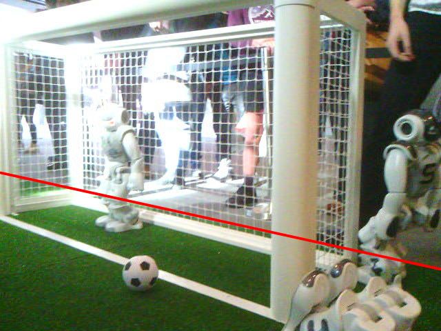
They operate with no preprocessing and only little post processing. In principle,
they do not need a separate field boundary detection because they already have
access to image context that should prevent them from detecting objects outside
the field. If the field boundary is desired as a specific feature, either the method
of this paper can be integrated into the FCNN or a conventional method based
on the output of semantic field segmentation can be employed. However, if most
objects are detected using analytical methods anyway, the input image size can
be chosen much smaller and the upscaling part of a segmentation network is not
necessary, in order to reduce computational cost.
     This paper contributes (a) a full description, code and data of a convolutional
neural network approach to detect the field boundary which was previously men-
tioned without details in a team report [15], and (b) the combination with the
prediction of confidence scores which can act as weighting factors in line model
fitting. The paper continues as follows: Section 2 reviews related work on the
topic of field boundary detection in robot soccer, section 3 describes our methods
in detail, section 4 evaluates the approach and presents the results, and section 5
concludes this paper.

2    Related Work

A classic approach to detect the field boundary consists of three steps: Firstly,
a classifier for pixel colors is established. Secondly, spots on the field boundary
are determined. Thirdly, a model of line segments is fitted through these spots.
There have been many implementations of this pattern, each differing in details.
     Reinhardt [9] first estimates the field color from channel-wise histograms
over the entire subsampled image. Then, the image is split into segments along
scan lines at edges in the luminance channel. Segments are classified into the
categories field, line or unknown. An unknown segment above a field segment
creates a candidate spot (i. e. there can be multiple spots per scan line). In order
to reject outliers, e. g. from a neighboring field, an iterative convex hull algorithm
evaluates multiple hypotheses and the one supported by most spots is chosen.
     Qian and Lee [8] start by sampling a guess of the field color near the robot’s
own feet, assuming that the majority of pixels there always belongs to the field.
Candidate boundary spots are generated by scanning downwards from the hori-
zon and choosing the spot where the difference in the number of visited green
and non-green pixels reaches its minimum. Finally, a model of one or two per-
pendicular lines is fitted using RANSAC.
     Fiedler et al. [4] include a field boundary detection in their vision pipeline.
Green pixels are masked based on a pre-calibrated seed that is dynamically
adjusted using a field boundary that is calculated from the previous field color
estimate, creating feedback loop. Depending on the camera angle, either the
topmost green pixel or the bottommost non green pixel (applying a low pass
filter in order to skip field lines) is chosen as candidate spot per vertical scan
line. Over these spots, the convex hull is computed to remove gaps caused by
occlusion of the field boundary by other players.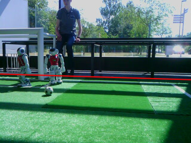
However, CNN-based approaches have also been proposed: Mahmoudi
et al. [7] describe a network that predicts five vertices of a polygon which bounds
the field. They use a 128 × 128 HSV image as input, followed by three pairs of
convolutional and pooling layers, and two fully connected layers in the end.
However, no quantitative results are given.
    Finally, Tilgner et al. [15] shortly mention in their team report that they de-
tect the field boundary using a deep neural network. The properties mentioned
there are 40 × 30 YCbCr images as input, a CNN architecture based on four
Inception-v2 blocks, and an output size matching the width of the input. Ap-
parently, they have successfully used the results at RoboCup 2019. This paper
started as an attempt to reproduce their approach.

3     Approach

In this section, the details of our approach are given. In general, like in [15] the
network takes a 40 × 30 image (downsampled from the full camera resolution) as
input and predicts 40 outputs, one per image column. Each output is the ratio
of the image height at which the field ends in the column that it represents,
i. e. 0 means that the field boundary is at or above the image and 1 means that
the field boundary is at or below image (i. e. the column does not contain any
field). In contrast to Mahmoudi et al. [7], who predict the vertices of a polygon
in the image, this is potentially less sensitive to small errors in the predictions
and allows for later regression (cf. section 3.5) to attenuate errors even more.

3.1   Dataset

Our dataset consists of images taken by the upper camera of NAO V6s. They
come from green RoboCup Standard Platform League fields in ten different
locations, including dark indoor environments (which also means that the images
are blurred due to high exposure times) as well as outdoor environments with
uneven natural lighting. The images have been JPEG-compressed and logged
by our robots during actual games, so there is occlusion by robots and all other
real-world effects. In order to reduce redundancy in the data, only about one
image per second has been kept.
    The resulting set of 36399 images, some of which are shown in fig. 1, has
been manually labeled with a custom tool. The annotation tool allows to mark
the field boundary as up to two lines by selecting two boundary points per line.
The labels are represented by the vertical coordinates at the left and right image
border as well as the location of the intersection of both lines, if it exists. This
means that we do not handle the case of two or more field corners in the image,
which only happens very rarely on a NAO due to the relation of the field size
and the camera’s horizontal field of view.
    For this work, the set is split into three parts: a training set of 28641 real
images and 4219 computer-generated images with ground-truth labels using a
derivative of UERoboCup [5], a validation set of 3449 real images and a test set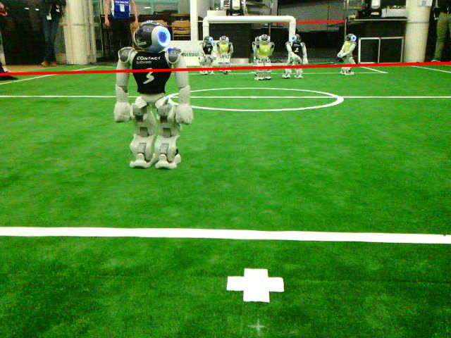
Fig. 1: Examples from the set of labeled real images

of 4309 images. The images in the validation set come from a location that is
not present the training set, and the test set includes yet more locations. The
complete dataset is publicly available.4

3.2    Model Architecture

As in [15], the architecture is based on four Inception-v2 [13] blocks. Each block
is divided into three N -filter branches which are concatenated in the end to
3N channels. The first branch starts by quartering the number of channels in a
pointwise Conv+BN+ReLU block. The following 3 × 3 Conv+BN+ReLU each
double the number of channels back to N and aggregate information from the
neighborhood. The second branch is similar to the the first one, but with only
one 3 × 3 Conv+BN+ReLU block. The third branch consists of a 3 × 3 max
pooling, followed by a pointwise Conv+BN+ReLU block. All blocks divide the
vertical resolution by two via strides, while keeping the number of columns.
    When the vertical size has been reduced to two rows after four blocks, a final
convolution layer aggregates all 2 · 3N channels within a column to O output
channels, i. e. it can also be seen as a fully connected layer with identical weights
per column. In each block, the horizontal receptive area is increased by 2 from
the two successive 3 × 3 convolutions in the first branch. This means that in
the end, each column output can contain information from 8 neighboring input
columns to both sides and is not restricted to data from its own column. The
architecture is depicted in fig. 2.
4
    https://sibylle.informatik.uni-bremen.de/public/datasets/fieldboundary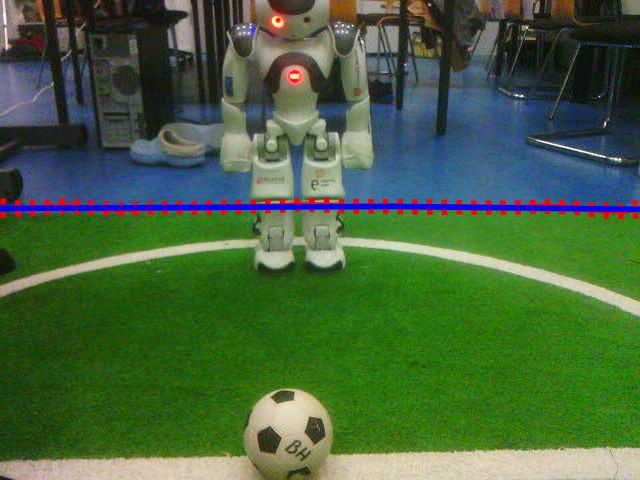
30 x 40 x [3, 1] Input                                N Filter Inception Block
                                                                       Input

Stage 1

   N Filter Inception Block     N/4 Filter 1x1 2D-Conv,       N/2 Filter 1x1 2D-Conv,         3x3 MaxPooling,
                               1x1 Strides, valid padding    1x1 Strides, valid padding   2x1 Strides, same padding

                                  Batch Normalization          Batch Normalization
Stage 2
                                         ReLU                          ReLU
   N Filter Inception Block

                                N/2 Filter 3x3 2D-Conv,       N Filter 3x3 2D-Conv,         N Filter 1x1 2D-Conv,
                               1x1 Strides, same padding    2x1 Strides, same padding     1x1 Strides, same padding
Stage 3

   N Filter Inception Block       Batch Normalization          Batch Normalization           Batch Normalization

                                         ReLU                          ReLU                        ReLU

Stage 4

   N Filter Inception Block      N Filter 3x3 2D-Conv,
                               2x1 Strides, same padding

                                  Batch Normalization

  O Filter 2x1 2D-Conv, 1x1
    Strides, valid padding               ReLU

                                                                   Concatenate
          40 x O Output

                               Fig. 2: Architecture of the CNN

3.3       Training
The network is trained in batches of 16 elements using the Adam algorithm with
Nesterov momentum [3] for up to 50 epochs. Training is stopped early when
the validation loss has not improved for five epochs. In the basic configuration
without predicting uncertainty (see section 3.4), the loss is defined as the mean
absolute difference between predicted and true vertical coordinate per column.
The learning rate starts at 0.001 and is quartered when there is no significant
improvement in validation loss for three epochs.
    Each batch of training data is augmented online before being fed into the
network. For this, we use imgaug [6] with several global and point-wise operators,
including flipping and cropping the image, adding noise and a constant brightness
offset, as well as motion blur. In addition, a custom augmentation that randomly
selects polygonal regions of the image and randomly scales their brightness in
order to model hard shadows [1] is applied.

3.4       Predicting Uncertainty
In some cases, it is impossible to determine the location of the field boundary at
a specific column in the image. For example, if the field boundary is occluded at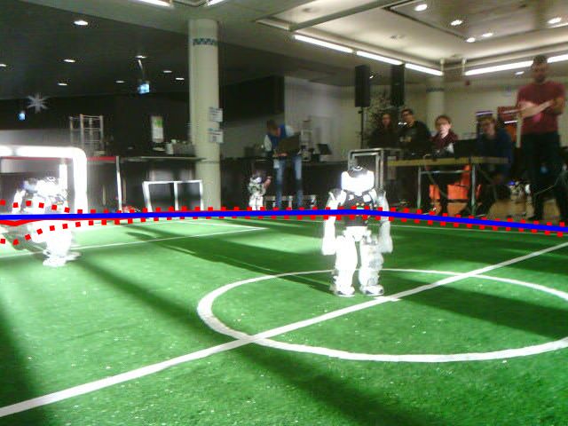
one of the image borders, there could be a corner behind it or not. However, the
network could actually see in the image that the predictions in those columns are
uncertain. Therefore, we employ the approach as in Richter-Klug and Frese [10]
to let the network predict its own uncertainty without needing additional la-
bels. Instead of predicting just a vertical coordinate, the network predicts the
parameters of a one-dimensional Gaussian distribution for each column.
    This can be achieved by using as loss function the negative log-likelihood of a
Gaussian parameterized by mean µ̂ and variance σ̂ 2 as predicted by the network,
evaluated at the true y-coordinate for a given column:

                     L(y, (µ̂, σ̂)) = − log p(y|µ̂, σ̂ 2 )
                                               1           (y−µ̂)2
                                    = − log √         e− 2σ̂2
                                              2πσ̂ 2
                                      log 2π                (y − µ̂)2
                                    =        + log σ̂ +
                                         2                     2σ̂ 2
                                                                                   1
Rewriting in terms of the reciprocal of the variance, the information ω̂ 2 =      σ̂ 2
(which our network actually predicts) yields

                                     log 2π            (y − µ̂)2 · ω̂ 2
                  L(y, (µ̂, ω̂)) =          − log ω̂ +                  .
                                        2                    2
This loss function can be interpreted in the following way: In order to minimize
the − log ω̂ term, the information must be maximized. At the same time, the
error of the predicted mean (y − µ̂)2 is scaled by this number, so in order to
simultaneously reduce that term, the mean prediction µ̂ must be moved closer
to the true label y. This way, ω̂ is guided to neither over- nor underestimate the
error of µ̂.                                     √
    In fact, the raw output of the network is ω̂ in order to ensure that ω̂ is
always nonnegative. Furthermore, we add a small value  to the argument of the
− log ω̂ term to shift it away from the singularity at 0. Also, the log-likelihood
loss is used in addition to the absolute coordinate difference |y − µ̂|, which should
put a bit more emphasis on actual accuracy.

3.5   Post Processing

In the simplest case, the coordinates predicted by the neural network can be used
directly as a polygonal chain. However, we can enhance the prediction by fitting
a model to the predicted values. Algorithm 1 describes a possible procedure to
fit up to two lines, which is enough for typical images taken by a NAO on a
standard platform league field. It takes advantage of the predicted ω̂ by using
it as weighting factor in the regression objective. This way, columns in which
the network is uncertain about its µ̂ prediction (i. e. ω̂ is low) do not contribute
much to the overall cost to be minimized.
    On a real robot, instead of selecting the model with lowest line fitting residual
c, one could also use the deviation of the angle between the two lines projected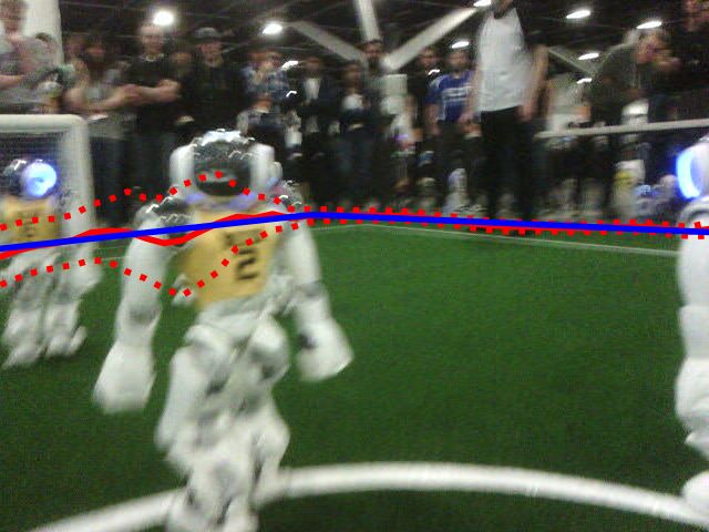
Algorithm 1 Fitting a model through predicted boundary spots using weighted
linear regression and exhaustive search for the apex.
 1:   function FitLine(X
                       P = (x1..k , µ̂1..k , ω̂1..k ))
 2:      C := (m, b) 7→ ki=1 ω̂i2 · (mxi + b − µ̂i )2
 3:      L ← arg minm,b C(m, b)
 4:      return (L, C(L))
 5:   end function
 6:
 7:   function FitModel(X = (x1..N , µ̂1..N , ω̂1..N ))
 8:      M ∗ , c∗ ←FitLine(X)
 9:      for i = 2 to N − 2 do
10:          LA , cA ←FitLine(X1..i )
11:          LB , cB ←FitLine(Xi+1..N )
12:          if cA + cB < c∗ then
13:               c∗ ← cA + cB
14:               M ∗ ← (LA , LB )
15:          end if
16:      end for
17:      return M ∗
18:   end function

on the ground (using the camera pose) from 90◦ . If no two lines have an angle
close to 90◦ the single line through all points is accepted.
     In principle, this method can be extended to cameras with wide-angle lenses
with distortion by choosing an appropriate model function. However, as soon as
it frequently happens that more than one field corner is in the image, searching
for them becomes more complex, e. g. quadratic for two corners.
     In addition, if ω̂ is low for most columns, i. e. the network is overall uncertain,
it can be assumed that the field boundary is not in the image at all (e. g. because
another robot is standing directly in front of the camera).

4      Evaluation

This section describes the experiments done to evaluate the approach and their
results. We have created 12 different versions of the CNN: combinations of three
different filter numbers N ∈ 8, 16, 24, grayscale or color input, and with or
without uncertainty prediction. The networks without uncertainty prediction
differ in that they have only one output channel which is the target coordinate,
and that this output is only trained on the mean absolute error as described in
section 3.3.

4.1     Accuracy

The first experiment for evaluating the accuracy of the method is to calculate
the mean absolute difference between predicted and true vertical field boundary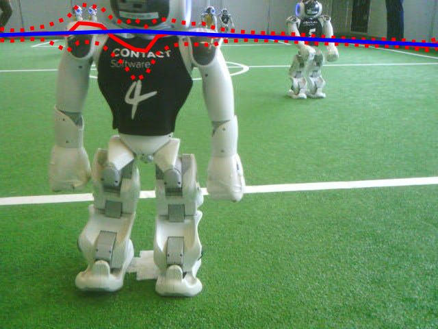
location over all columns in the test set. For interpreting these numbers, recall
that the network operates on an input that is 30 pixels high, so an error of one
pixel corresponds to 0.03333. The results are given in table 1. It is noticeable
that all color networks are consistently better than their grayscale counterpart.
This is not surprising, as the green color is the main feature of the field. Also, for
each column in table 1, the performance improves with the number of filters per
branch N . Increasing N even further, e. g. to 32, also increases the number of
parameters in the network, e. g. to about 60000 for N = 32, and is therefore not
desirable. Using different filter numbers per block is possible too, but expands
the design space a lot. The counterparts with uncertainty prediction are, with
one exception5 , significantly worse than the networks which have been trained to
predict the coordinate only. This is understandable in the way that they actually
have been trained for a different objective.
Table 1: Mean absolute error of raw network output on the test set
Without Uncertainty With Uncertainty
Grayscale Color Grayscale Color
N =8 0.05708 0.03108 0.06061 0.03800
N = 16 0.05412 0.02357 0.05110 0.03168
N = 24 0.03998 0.02355 0.04734 0.02781
Next, we evaluate the performance after model fitting according to sec-
tion 3.5. Here, the mean absolute error is determined after discretizing the fitted
model in the same way as the labels are, so the numbers in table 2 are compara-
ble to table 1. The fitting for the networks without uncertainty prediction assigns
a unit weight to all columns. For comparison, results in which unit weights are
used are also included for the color networks with uncertainty. In all 12 con-
figurations, the error has been reduced by line fitting with respect to the raw
outputs from table 1. However, the errors of the models fitted with weighting
factors predicted by the network are still worse than those fitted through the
outputs of a network that has been trained to predict the coordinate only. On the
other hand, there is an improvement in the uncertainty models when using the
predicted instead of unit weights (i. e. from the rightmost column of table 2 to
the one next to it), indicating that the predicted uncertainty actually correlates
with the positional accuracy of the network in a specific image column.
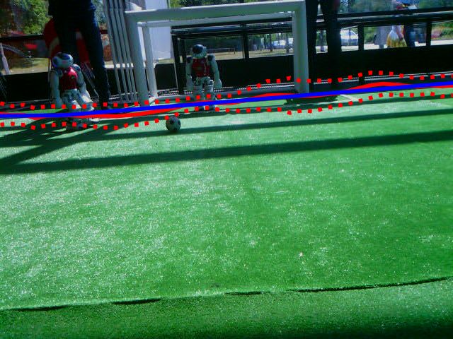
For a visual evaluation of the networks with uncertainty prediction, N = 24
and line fitting, refer to fig. 3. All nine images are neither in the training nor in
5
The optimization for the combination without uncertainty, grayscale, N = 16 stopped
after only 9 epochs.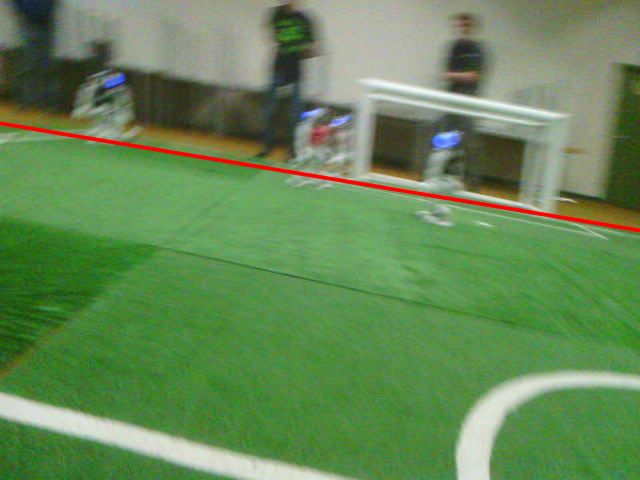
Table 2: Mean absolute error of fitted models on the test set

            Without Uncertainty                     With Uncertainty
            Grayscale      Color         Grayscale    Color      Color Unweighted

N =8         0.05271      0.02907         0.05293    0.03374         0.03665
N = 16       0.05060      0.02226         0.04431    0.02727         0.03037
N = 24       0.03718      0.02226         0.04123    0.02436         0.02668

the validation set. While the neural network using colors looks quite accurate,
the performance on grayscale images is significantly worse. Occlusion of the
field boundary from robots often causes the mean prediction to deviate, but the
uncertainty reflects this well, as can be seen, e. g., in the leftmost image in the
fourth row.
    A frequent artifact are arcs at the borders of the image, i. e. the left-
/rightmost few columns deviate increasingly from the actual field boundary. We
hypothesize that this is due to the zero padding which causes the outer columns
to receive less activation. However, the uncertainty also correctly increases there.
A column-specific bias could help with this.

4.2   Inference Time
In order to run our networks on a NAO V6, we use CompiledNN [14]. The num-
bers in table 3 have been obtained using the included benchmark tool with 10000
iterations. The inference times are mainly influenced by the number of filters N .
The usage of color in the input adds 20 µs on average, while the additional out-
put channel for predicting uncertainty has no significant impact. Anyway, all
networks are fast enough to be used as a preprocessing step of a real-time 30 Hz
vision pipeline.

      Table 3: Inference times of the CNNs on a NAO V6 in milliseconds

                        Without Uncertainty          With Uncertainty
                        Grayscale    Color           Grayscale     Color

           N =8           0.555       0.573            0.558       0.572
           N = 16         1.539       1.557            1.533       1.562
           N = 24         3.198       3.223            3.204       3.218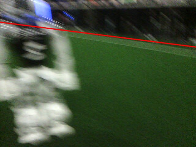
Fig. 3: Grayscale/color image pairs with the output of the respective networks
with uncertainty and N = 24. The solid red line is the predicted mean, the
dotted lines are ±σ̂ intervals, and the blue line is the fitted model.
5   Conclusion
In this paper, we expanded on [15] and showed that a convolutional neural net-
work is able to detect the field boundary in an image from raw pixels to column-
wise vertical coordinates. Color information is important for this to work prop-
erly. The overall accuracy is reasonably good also in difficult conditions, as can
be seen in fig. 3. Results about uncertainty prediction are inconclusive: Numeri-
cal results even after weighted line fitting are not as good as the plain coordinate
predictions of networks which do not predict uncertainty, but at least for the net-
works with uncertainty output, the weighted line fitting is more accurate than
with unit weights. To combine the advantages of both variants, it can be exam-
ined to pretrain a network without the uncertainty output and then introduce
the additional output while freezing some of the layers. The inference times of
all presented networks are low enough to be used in a real-time vision pipeline.
    Some of the presented networks are used by the SPL team B-Human. They
apply different postprocessing that also transfers information between the two
cameras of the NAO, but uses the uncertainty prediction only for determining
whether the field boundary is in the image at all. It has already been used in
test games and the German Open Replacement Event 2021 and will be used at
RoboCup 2021.
    For future investigation, we have started experiments to replace the CNN by
a transformer, similar to [2]. The prototype treats each column of the image as
an element in a sequence, such that in the end, the results can be read from
a regression head for each element. The idea is that the transformer is more
able to combine global features while retaining the column-wise structure of
the problem, but without being restricted to the receptive field of convolutions.
However, we cannot report results yet.
    The code as well as the dataset that have been used for this paper are avail-
able online: https://github.com/bhuman/DeepFieldBoundary

Acknowledgements
This work is partially funded by the German BMBF - Bundesministerium für
Bildung und Forschung project Fast&Slow (FKZ 01IS19072). Furthermore, the
authors would like to thank the past and current members of the team B-Human
for developing the software base for this work.

References
 1. Blumenkamp, J., Baude, A., Laue, T.: Closing the reality gap with unsupervised
    sim-to-real image translation for semantic segmentation in robot soccer (2019),
    https://arxiv.org/abs/1911.01529
 2. Dosovitskiy, A., Beyer, L., Kolesnikov, A., Weissenborn, D., Zhai, X., Unterthiner,
    T., Dehghani, M., Minderer, M., Heigold, G., Gelly, S., Uszkoreit, J., Houlsby,
    N.: An image is worth 16x16 words: Transformers for image recognition at scale
    (2020), https://arxiv.org/abs/2010.11929
3. Dozat, T.: Incorporating Nesterov momentum into Adam. In: ICLR Workshop
(2016)
4. Fiedler, N., Brandt, H., Gutsche, J., Vahl, F., Hagge, J., Bestmann, M.: An open
source vision pipeline approach for RoboCup humanoid soccer. In: Chalup, S.,
Niemueller, T., Suthakorn, J., Williams, M.A. (eds.) RoboCup 2019: Robot World
Cup XXIII. LNCS, vol. 11531, pp. 376–386. Springer (2019)
5. Hess, T., Mundt, M., Weis, T., Ramesh, V.: Large-scale stochastic scene generation
and semantic annotation for deep convolutional neural network training in the
RoboCup SPL. In: Akiyama, H., Obst, O., Sammut, C., Tonidandel, F. (eds.)
RoboCup 2017: Robot World Cup XXI. LNCS, vol. 11175, pp. 33–44. Springer
(2018)
6. Jung, A.B., Wada, K., Crall, J., Tanaka, S., Graving, J., Reinders, C., Yadav, S.,
Banerjee, J., Vecsei, G., Kraft, A., Rui, Z., Borovec, J., Vallentin, C., Zhydenko,
S., Pfeiffer, K., Cook, B., Fernández, I., De Rainville, F.M., Weng, C.H., Ayala-
Acevedo, A., Meudec, R., Laporte, M., et al.: imgaug (2020), https://github.
com/aleju/imgaug
7. Mahmoudi, H., Fatehi, A., Gholami, A., Delavaran, M.H., Khatibi, S., Alaee, B.,
Tafazol, S., Abbasi, M., Doust, M.Y., Jafari, A., Teimouri, M.: MRL team descrip-
tion paper for humanoid KidSize league of RoboCup 2019. Tech. rep., Mechatronics
Research Lab, Qazvin Islamic Azad University (2019)
8. Qian, Y., Lee, D.D.: Adaptive field detection and localization in robot soccer. In:
Behnke, S., Sheh, R., Sarıel, S., Lee, D.D. (eds.) RoboCup 2016: Robot World Cup
XX. LNCS, vol. 9776, pp. 218–229. Springer (2017)
9. Reinhardt, T.: Kalibrierungsfreie Bildverarbeitungsalgorithmen zur echtzeitfähigen
Objekterkennung im Roboterfußball. Master’s thesis, Hochschule für Technik,
Wirtschaft und Kultur Leipzig (2011)
10. Richter-Klug, J., Frese, U.: Towards meaningful uncertainty information for CNN
based 6d pose estimates. In: Tzovaras, D., Giakoumis, D., Vincze, M., Argyros, A.
(eds.) Computer Vision Systems. LNCS, vol. 11754, pp. 408–422. Springer (2019)
11. Rodriguez, D., Farazi, H., Ficht, G., Pavlichenko, D., Brandenburger, A., Hosseini,
M., Kosenko, O., Schreiber, M., Missura, M., Behnke, S.: RoboCup 2019 AdultSize
winner NimbRo: Deep learning perception, in-walk kick, push recovery, and team
play capabilities. In: Chalup, S., Niemueller, T., Suthakorn, J., Williams, M.A.
(eds.) RoboCup 2019: Robot World Cup XXIII. LNCS, vol. 11531, pp. 631–645.
Springer (2019)
12. Schnekenburger, F., Scharffenberg, M., Wülker, M., Hochberg, U., Dorer, K.: De-
tection and localization of features on a soccer field with feedforward fully convo-
lutional neural networks (FCNN) for the adult-size humanoid robot Sweaty. In:
Proceedings of the 12th Workshop on Humanoid Soccer Robots, IEEE-RAS Inter-
national Conference on Humanoid Robots. Birmingham (2017)
13. Szegedy, C., Vanhoucke, V., Ioffe, S., Shlens, J., Wojna, Z.: Rethinking the In-
ception architecture for computer vision (2015), https://arxiv.org/abs/1512.
00567v3
14. Thielke, F., Hasselbring, A.: A JIT compiler for neural network inference. In:
Chalup, S., Niemueller, T., Suthakorn, J., Williams, M.A. (eds.) RoboCup 2019:
Robot World Cup XXIII. LNCS, vol. 11531, pp. 448–456. Springer (2019)
15. Tilgner, R., Reinhardt, T., Seering, S., Kalbitz, T., Eckermann, S., Wünsch, M.,
Mewes, F., Jagla, T., Bischoff, S., Gümpel, C., Jenkel, M., Kluge, A., Wieprich,
T., Loos, F.: Nao-Team HTWK team research report. Tech. rep., Hochschule für
Technik, Wirtschaft und Kultur Leipzig (2020)You can also read