Testing quantum speedups in exciton transport through a photosynthetic complex using quantum stochastic walks
←
→
Page content transcription
If your browser does not render page correctly, please read the page content below

Testing quantum speedups in exciton transport through a photosynthetic complex using quantum
stochastic walks
Pratyush Kumar Sahoo1 and Colin Benjamin2
1 Department of Physical Sciences, Indian Institute of Science Education & Research, Kolkata, India
2 School of Physical Sciences, National Institute of Science Education & Research, HBNI, Jatni-752050, India∗
Photosynthesis is a highly efficient process, nearly 100 percent of the red photons falling on the surface of
leaves reach the reaction center and get transformed into energy. Quantum coherence has been speculated to
play a significant role in this very efficient transport process which involves photons transforming to exciton’s
and then traveling to the reaction center. Studies on photosynthetic complexes focus mainly on the Fenna-
arXiv:2004.02938v1 [cond-mat.stat-mech] 6 Apr 2020
Matthews-Olson complex obtained from green-sulfur bacteria. However, there has been a debate regarding
whether quantum coherence results in any speedup of the exciton transport process. To address this we model
exciton transport in FMO using a quantum stochastic walk(QSW) with either pure dephasing or with both
dephasing and incoherence. We find that the QSW model with pure dephasing leads to a substantial quantum
speedup as compared to a QSW model which includes both dephasing and incoherence.
I. INTRODUCTION in FMO. In Ref. [8] a more general form of quantum walk
called the quantum stochastic walk(QSW) which is adaptable
The first step of photosynthesis takes place via the an- to include classical effects either only dephasing or both inco-
tennae molecules called the chromophores. These antennae herence and dephasing was introduced. A QSW interpolates
molecules loose electrons when light falls on them and an between classical random walk(CRW) and continuous-time
electron-hole pair or exciton is formed[1]. This exciton in turn quantum walk (CTQW) through a single parameter ω. ω is a
has to reach the reaction center where the charge separation measure of the amount of dephasing and/or incoherence built
occurs and energy is stored. Usually these reaction centers into the QSW. Later in Ref. [9] QSW was used to model FMO
are far in terms of molecular distance from the excited anten- and results were compared with Ref. [7]. Our main aim in this
nae molecule. But, this process of transferring the captured paper is to test the prognosis that quantum effects do not lead
photon to the reaction centre is seen to exhibit an efficiency to any speedup of the exciton transport from antenna to reac-
close to 100 percent. In 2007, it was reported[2] using "two tion center as was advanced in Ref. [7]. Quantum speedup of
dimensional Fourier transform electronic spectroscopy" (2D- excitonic transport is measured via the localization time(tloc ).
FTES) that quantum coherence could be playing an important Localization time[7] is defined as time at which the onset of
role in the exciton transport in Fenna-Matthews-Olson (FMO) sub-diffusive transport occurs in the exciton transport process.
complex found in green-sulphur bacteria. Later this was theo- The greater is the localization time, the more is the duration
retically analyzed[3]. The exciton thus must not be following for which super-diffusive transport prevails. Thus, for sig-
a classical random walk to get to the reaction center before its nificant speed up localization time must be large. In Ref. [7]
conversion to energy[1] rather the antennae molecules were localization time at both 77K and 300K is around 70 f s. In our
operating via a search strategy called the quantum walk[3]. A work, on the other hand, we find for the QSW model with pure
quantum walker takes all possible paths, (like a superposed dephasing localization time at 300K is more than that at 77K
atom in the two-slit experiment) as opposed to classical ran- in accordance with the expectation of a quantum speedup. The
dom walker who must choose a single route. This gives quan- main take home message of this work is that at life sustaining
tum walk an advantage in the sense that it spreads with rate temperatures of 300K, the QSW model with pure dephasing
proportional to the time taken as compared to classical ran- leads to quantum speedup in exciton transport while in case
dom walk which spreads as square root of time. Quantum of a QSW model with both dephasing and incoherence or the
coherence in FMO complex implies exciton transfer seen at master equation approach of Hoyer, et. al., in Ref. [7] there is
life sustaining temperatures of 300K is aided by the quan- no quantum speedup seen at 300K.
tum walk process which apparently takes place in presence
The outline of the paper is as follows: in the next section
of dephasing. Later in 2010, it was demonstrated[2] that
we give details of the quantum stochastic walk used to model
quantum coherence was seen for nearly 300 f s in FMO com-
exciton transport in FMO and introduce the two models, one
plex at 300K. Quantum coherence at normal ambient tem-
on incorporating pure dephasing in QSW and the other on in-
peratures have also been detected in LHC2 complex found in
cluding both incoherence and dephasing in the QSW. Subse-
bacteria[4], in spinach[5] and in a group of aquatic algae[6].
quent to this we give details of the FMO complex, it’s Hamil-
In Ref. [3] quantum walks were first used to study exciton
tonian and on how both QSW models are used to model ex-
transfer dynamics in FMO complex interacting with a thermal
citon transport in FMO. In section III we plot the results of
bath. Later, Hoyer, et. al., in Ref. [7] used a master equa-
our simulations for total site coherence, site population, mean
tion approach with pure dephasing to model exciton transfer
square displacement and localization time. In section IV we
discuss our results and plots via two tables, the first for local-
ization time and the second for other quantities. We end the
∗ colin.nano@gmail.com paper and section IV with conclusion which includes a per-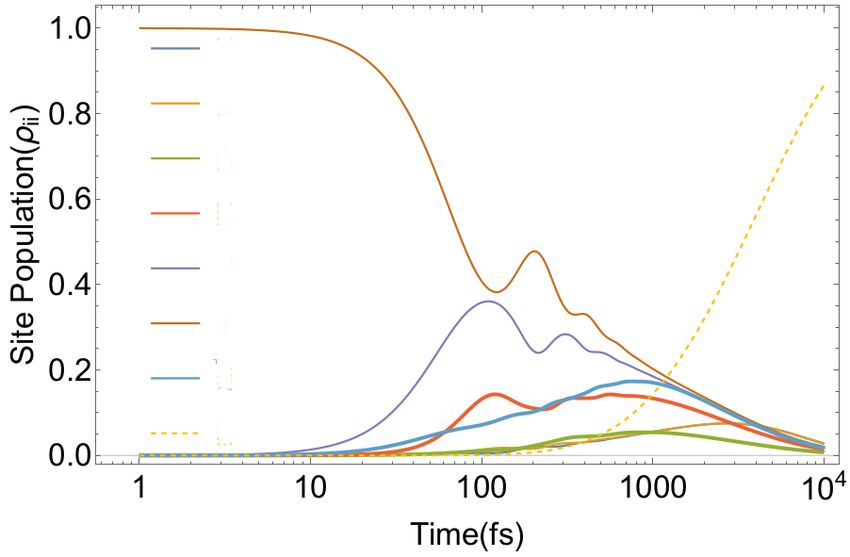
2

spective on future endeavors in this area.                             On the other hand, when modeling a QSW with both de-
                                                                    phasing and incoherence, the Lindblad operators are chosen
                                                                    to be, (see also [8] and section 2 of Ref. [9])-
           II.   QUANTUM STOCHASTIC WALK                                                         q
                                                                                           L̂k = |Hi j | |iih j|,          (4)
   Two variants of quantum walks are known- discrete-time           with Hi j = hi| H | ji being the matrix elements of the Hamil-
quantum walk (DTQW)[10] and continuous time quantum                 tonian operator H. The Lindblad operators in Eq. 4 repre-
walk (CTQW)[11]. A more general form of continuous time             sent scattering between all pair of vertices. For ω = 1, the
quantum walk called the quantum stochastic walk (QSW) was           QSW model with both dephasing and incoherence reduces to
first introduced in Ref. [8]. It has the advantage of interpolat-   CRW[7].
ing continuously from a classical random walk to a continuous
time quantum walk and can address quantum walk processes
which are coupled to an environment. QSW was derived from                  III.   MODELING EXCITON TRANSPORT IN FMO
Kossakowski-Lindblad master equation[12, 13], which is used                                 COMPLEX
to describe quantum stochastic process and model open quan-
tum systems. QSW is based on density matrix, dynamics of               In the photosynthetic process, energy gathered from light
which is given by[8]-                                               by antennae molecules is transmitted across the network of
                                                                    chlorophyll molecules to reaction centers [15]. This process
   dρ(t)                                                            is nearly 100% efficient as nearly all the red photons are
         = − (1 − ω) i [H, ρ(t)]
    dt                                                              captured and stored as energy. Experiments have revealed
              K                                                  long-lasting quantum coherence in energy transport across a
                           †    1 †                  †
         + ω ∑ L̂k ρ(t)L̂k −      L̂ L̂k ρ(t) + ρ(t)L̂k L̂k (1)     range of photosynthetic light-harvesting complexes[16–20].
            k=1                 2 k
                                                                    One such light-harvesting complex is the Fenna-Matthews-
where ρ(t) is the density matrix representation of walker at        Olson (FMO) complex from the green sulphur bacteria. The
time t. For QSW on any graph G, ρ(t) is a N × N matrix              FMO complex consists of seven regions called chromophores,
with vertex states- {|1i , ..., |Ni} as the basis, and elements     through which the exciton’s propagate via hopping and it
ρi j (t) = hi| ρ(t) | ji. 0 ≤ ω ≤ 1 is a parameter which interpo-   has been speculated that this propagation is aided by phase
lates between CRW and CTQW. For ω = 0 both models of                coherence[16].
QSW considered, reduce to a CTQW. H is the Hamiltonian
operator responsible for coherent dynamics. The index k has
                                                                      A.     Understanding exciton transport in FMO: the model of
a unique value for each pair of i, j implying k has N 2 unique
                                                                                             Hoyer, et. al.,[7]
values, N being the number of vertices in the graph. The first
term on the right hand side is responsible for coherent dy-
namics and the second term on right gives rise to incoherent           To understand how quantum effects are important in the
dynamics via either only dephasing or both dephasing and in-        very efficient transfer of excitons at room temperatures,
coherent scattering.                                                Hoyer, et. al.,in Ref. [7] used a master equation approach to
    L̂k are Lindblad operators which are sparse N × N matrices.     model exciton transport in FMO by incorporating dephasing
N being the total number of vertices of the underlying graph.       into their model. The plot of total site coherence (Fig. 3(c)
For the purpose of modeling a QSW with only pure dephasing,         of [7]) for both 77K and 300K indicates the presence of co-
the Lindblad operators are (see section 4.2 of Ref. [9] and         herence for nearly 500 f s. Despite this long lived coherence,
Refs. [8, 14] for more details on modeling QSW with pure            the plot of power law of mean square displacement(Fig. 3(b)
dephasing):                                                         of [7]) indicates that much of the transport occurs in the sub-
                                                                    diffusive regime. The super-diffusive nature of transport lasts
                              p                                     for only 70 f s, indicating localization time of 70 f s at both
                      L̂k =       |Hii | | iihi |.           (2)
                                                                    temperatures of 77K and 300K. Hence, Hoyer, et. al., in
                                                                    Ref. [7] conclude that coherence in FMO does not yield dy-
wherein Hii = hi| H |ii are the diagonal elements in the matrix
                                                                    namic speed up unlike that seen in quantum search algorithms,
representation of Hamiltonian operator H. In this model we
                                                                    even though quantum coherence may last longer. The main
have Lindblad operators corresponding to the diagonal entries
                                                                    conclusion of Ref. [7] was quantum coherent effects in a bi-
of the density matrix. For ω = 1 it can be shown[9] that:
                                                                    ological system like FMO lead to optimized or robust exci-
                             (                                      ton transport, which is 100% efficient rather than any speedup
                 dρi j (t)     −ρi j (t), i , j                     of the transport. In this work we test this conclusion regard-
                           =                                (3)
                    dt         0,         i= j                      ing speedup of the exciton transport via quantum stochas-
                                                                    tic walks(QSW). To this end, we employ two different ap-
Equation (3) shows that the off-diagonal terms of the density       proaches for incorporating incoherence into the QSW, the first
matrix which represent coherences die exponentially while the       pure dephasing (see Eq. (2)) and the second dephasing with
population(ρii ) remains constant. So, there is no transport at     incoherence (see Eq. (4)). Both the methods are explained in
ω = 1 limit for the pure dephasing model.                           greater detail in the subsequent sections.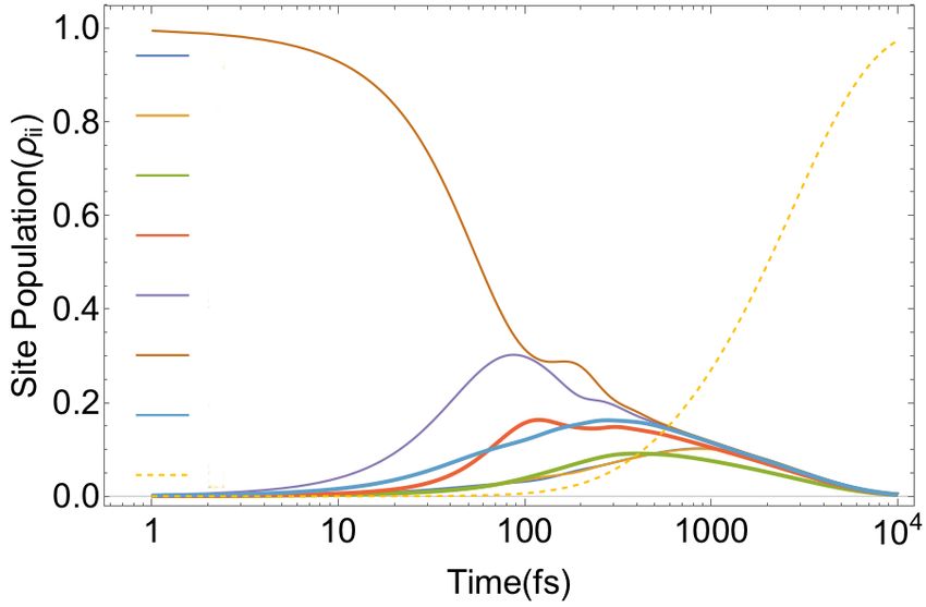
3
B. Modeling FMO using QSW
Earlier attempts [3, 7, 21] to model exciton transfer in FMO
complex have used non-probability conserving master equa-
tions. These equations use loss terms to model absorption
of exciton’s by reaction centers and like QSW combine inco-
herent and coherent transport via a master equation approach.
Here, we take another approach of adding an extra vertex and
model FMO using probability conserving QSW. This was first
done in Ref.[9]. This model is versatile and can reproduce
pure dephasing transport as well as both dephasing and inco-
Figure 1. Simplified figure of FMO complex. The chromophores are
herent scattering, however, it does not have an explicit tem-
numbered from 1 to 7. Vertex 8 is the sink. Exciton travels from site
perature dependence. Ref. [9] also made an incorrect compar- 6 and finds it’s way to site 3 the reaction center. The lines between
ison of the QSW model with both incoherence and dephasing the chromophore sites represent dipolar coupling between them. In
to the model of Ref. [7] which includes only dephasing. In fact, there is coupling between every site which is represented by
our work, we correct this and compare QSW with pure de- the Hamiltonian given in Eq. (6)[23]. But only the couplings above
phasing to the model of Ref. [7] to get a proper one to one 15cm−1 have been shown in Fig. 1, similar to Ref. [7]. One can
correspondence between ω and temperature. Thus, we com- assume the exciton to be following the path according to Fig. 1 with
pare the plots of total site coherence versus time for various sufficient confidence.
values of ω for QSW using pure dephasing with Fig. 3(c) of
Ref.[7]. We find that ω = 0.19 corresponds to a temperature
of 77K and ω = 0.486 corresponds to a temperature of 300K.
Using ω = 0.19 in the simulation of QSW with pure dephas- We use the Hamiltonian obtained by Adolphs and Renger[23]:
ing in FMO, the plot of site population versus time replicates
Fig. 3(d) of [7] which is at 77K. First in sub-section 3.B.1 we
−96 −4.4 4.7 −12.6 −6.2
model exciton transfer in FMO using pure dephasing, then in 200 5
−96 320 33.1 6.8 4.5 7.4 −0.3
sub-section 3.B.2 both dephasing and incoherent scattering is
5 33.1 0 −51.1 0.8 −8.4 7.6
considered. The QSW simulations shown in section IV use
H = −4.4 6.8 −51.1 110 −76.6 −14.2 −67
the QSWalk package[9, 22] for Wolfram Mathematica. 4.7
4.5 0.8 −76.6 270 78.3 −0.1
−12.6 7.4 −8.4 −14.2 78.3 420 38.3
−6.2 −0.3 7.6 −67 −0.1 38.3 230
(6)
The units of energy are cm−1 (we follow the usual spec-
troscopy convention of expressing energy in terms of the
wavelength of photon with that energy, i.e., 1cm−1 ≡
1. Modeling exciton transport in FMO via QSW with pure
1.23984 × 10⁻⁴ eV ). The model uses the above Hamilto-
dephasing
nian, padded with zeros to construct an 8 × 8 matrix, so as
to describe coherent evolution. For QSW using pure de-
phasingpwe use the Lindblad operators- defined as in Eq. 2
FMO has 7 chromophore sites (see Fig.1). The excitation
L̂k = |Hii ||iihi|. There is an unique value of k for each
starts at initial site 6 and gets absorbed at site 3[23], the reac-
vertex pair i, j. The sum in Eq. (5) extends over all i, j such
tion center. QSW is a probability conserving process, in con-
= N 2 . An extra Lindblad operator is used for the sink:
that k √
trast Hoyer, et. al.’s model[7] doesn’t conserve probability. To
L̂k = α|8ih3|, where α determines the rate of absorption at
have a one-to-one correspondence between both of our QSW
the sink (here α = 100 as in Ref.[9]). Through these Lindblad
models with the model of Hoyer, et. al., we include a sink to
operators we incorporate incoherent scattering as well as de-
model absorption. Therefore, in our QSW simulations, an ex-
phasing. The initial density matrix is given as ρ(0) = |6ih6|,
tra site numbered 8 is added, which acts as a sink, see Ref. [9].
assuming the initial excitation being localized at site 6. Since
This extra vertex is added using a directed edge and does not
temperature doesn’t appear in QSW we try to make a one to
take part in the coherent transport via the Hamiltonian. The
one correspondence between our simulation of the total site
time evolution of the density matrix for our QSW is given by:
coherence(see section IV.A below) with the same simulation
in Ref. [7]. This gives us the equivalent ω values for partic-
ular temperatures. ω = 0.19 corresponds to temperature of
dρ 77K and ω = 0.486 corresponds to 300K. This equivalence
= −(1 − ω)i[H, ρ(t)] between ω and temperature is got by comparing the plot of
dt
K
total site coherence Fig. 2(a) of this work, with Fig. 3(c) of
† 1 Ref. [7]. The procedure to calculate the total site coherence is
+ ω ∑ (L̂k ρ(t)L̂∗k − (L̂k† L̂k ρ(t) + ρ(t)L̂k† L̂k )) (5)
k=1 2 given in the next section.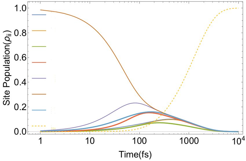
4

                                                                                                                 1.5
                                     2.0                                ω=0.19 (77K)                                                               ω=0.19 (77K)

              Total Site Coherence

                                                                                          Total Site Coherence
                                                                        ω=0.486 (300K)
                                                                                                                                                   ω=0.486 (300K)
                                     1.5                                                                         1.0

                                     1.0
                                                                                                                 0.5
                                     0.5

                                     0.0                                                                         0.0
                                           1           10       100      1000       104                                1           10      100      1000          104
                                                             time(fs)                                                                   time(fs)
                                                            (a)                                                                         (b)

Figure 2. Total site coherence versus time using (a) Pure dephasing (b) Dephasing and incoherent scattering. Comparing Fig. 2(a) with
Fig. 3(c) of Ref. [7], we get the equivalent values for ω at temperatures of 77K and 300K.

                                                   1                                                                           1

                                                   2                                                                           2

                                                   3                                                                           3

                                                   4                                                                           4

                                                   5                                                                           5

                                                   6                                                                           6

                                                   7                                                                           7

                                                   8                                                                           8

                                                            (a)                                                                         (b)

Figure 3. Site population(ρii ) versus time for pure dephasing at temperatures (a) 77K (ω = 0.19) (b) 300K (ω = 0.486). Fig. 3(a) is in excellent
agreement with Fig. 3(d) of Ref.[7].

                                               1                                                                           1

                                               2                                                                           2

                                               3                                                                           3

                                               4                                                                           4

                                               5                                                                           5

                                               6                                                                           6

                                               7                                                                           7

                                               8                                                                           8

                                                            (a)                                                                         (b)

    Figure 4. Site population(ρii ) versus time for dephasing and incoherence at temperatures (a) 77K (ω = 0.19) (b) 300K (ω = 0.486).

    2.   Modeling exciton transport in FMO via QSW with both                                                     of QSW as defined in [8] we get CRW (ω = 1) and CTQW
               dephasing and incoherent scattering                                                               (ω = 0) as two extreme cases. For the  √ sink we use the same
                                                                                                                 Lindblad operator as previous: L̂k = α|8ih3|, with α = 100
                                                                                                                 determining the absorption rate at the sink. We now make a
   For the case of QSW model with both dephasing and                                                             detailed study of exciton transport in FMO complex focusing
incoherence[8]
      p         we use the set of Lindblad operators, see Eq. 4,                                                 on total site coherence, site population, mean square displace-
L̂k = |Hi j ||iih j|. It is important to note that for this model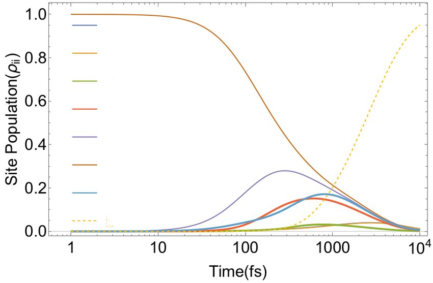
5

ment and localization time better understand the exciton dy-        The mean square displacement versus time has been plotted
namics of a FMO complex and compare with the results of             in Fig. 5 for both pure dephasing and dephasing with incoher-
Ref. [7] especially with regards to the localization time.          ence. By assuming that mean square displacement follows a
                                                                    power law, see Ref. [7] for reasons behind this assumption,
                                                                    we have
                           IV.   RESULTS
                                                                                  hx2 i = t b , and taking logarithm on both sides,
                     A.    Total Site Coherence                       we get- loghx2 i = b logt.                                  (8)
                                                                    where t denotes time. Exponent ’b’ versus time has been plot-
   Total site coherence is defined as sum of the absolute value     ted in Fig. 6, which has been obtained by plotting slope of
of each off-diagonal element of the density matrix in the site      log-log plot of mean square displacement (slope of Fig. 5).
basis. Finite valued off- diagonal elements of a density matrix     For b > 1 the transport is called super diffusive and b < 1 cor-
indicate coherence. Total site coherence is a measure of the        responds to sub-diffusive transport. These definitions are with
coherence present in the FMO complex. The QSW does not              respect to classical random walk (CRW) which follows dif-
have explicit temperature dependence. It has a single param-        fusive transport at b = 1. In Fig. 3(b) of Ref.[7] the plots of
eter ω and to get an explicit temperature dependence for our        power law versus time shows the transition from super diffu-
QSW model via ω we compare plots of total site coherence            sive to sub-diffusive transport at 70 f s for both 77K as well as
versus time (for pure dephasing) at different values of ω with      300K. In the plots of power law versus time for QSW with
Fig. 3(c) of Ref. [7] and find that ω = 0.19 corresponds to         pure dephasing (Fig. 6(a)) and QSW with both dephasing and
a temperature of 77K while ω = 0.486 corresponds to 300K            incoherence (Fig. 6(b)) shows that the time for this transition
(see Fig. 2(a) which depicts total site coherence for exciton       time is different at different temperatures (corresponding to
transport in QSW with pure dephasing). Ref. [7] uses mas-           different ω). More about this result has been explained in the
ter equation with pure dephasing to model exciton transfer in       next section on localization time. Further, the Mathematica
FMO. Hence the plot of total site coherence using QSW with          code and method of calculation for mean square displacement,
pure dephasing has been compared with the respective plot           power law b and localization time(tloc ) has been provided in
(Fig.3(c)) of Ref. [7] to obtain the correspondence between ω       Appendix A.
and temperature.

                                                                                         D.   Localization time
                          B.   Site Population
                                                                       The localization time(tloc ) is defined[7] as the time at which
   Site population of the ith site in the FMO complex is de-        the transition of power law b occurs from super diffusive to the
fined as ρthii element of the density matrix ρ. Site population     sub-diffusive regime, i.e., the power b goes below 1. tloc val-
of the ith site represents the probability of finding the exciton   ues have been given in Table I. We see that for the QSW model
at that site. Initially the exciton is at site 6. Using Eq. 2 and   with pure dephasing there is indeed a speed up at 300K as tloc
the Mathematica code(QSWalk[9, 22]), we calculate the time          increases at 300K(ω = 0.486) as compared to 77K(ω = 0.19).
evolution of the population of each site via QSW. Site popu-        Even if we change the initial state of the exciton to be at site
lation versus time for QSW with pure dephasing at both 77K          1 instead of site 6, we get speed up at 300K for the QSW
(i.e., ω = 0.19) and 300K (i.e., ω = 0.486) has been plotted        model with pure dephasing, the tloc values being 63 f s at 77K
in Fig. 3. Fig. 3(a) is in excellent qualitative agreement with     and 98 f s at 300K. This result is the key takeaway message of
Fig. 3(d) of Ref. [7]. We see that with increase in temperature     our work. However, in case of QSW model with both dephas-
the oscillations die down faster with time. Site population         ing and incoherence there is on the other hand a slow down
versus time for QSW with both incoherence and dephasing is          instead of speed up, tloc reduces from 54 f s at 77K to 15 f s
given in Fig. 4. Further, with incoherent scattering incorpo-       at 300K. These results are in stark contrast to that seen by
rated the oscillations in site population die out too(see Figures   Hoyer, et. al.’s work[7] where tloc doesn’t change from 77K
4(a) and 4(b)).                                                     to 300K. An explanation for these findings on localization
                                                                    time has been provided in Appendix B and Appendix C by
                                                                    comparing site population. One can clearly see in Fig. 8 (Ap-
                C.    Mean Square Displacement                      pendix B), that the exciton population at each site invariably
                                                                    reaches a peak at 300K later than that at 77K. Thus, time for
  Mean square displacement is defined as[7]                         ρii to peak at 77K is always less than the time for ρii to peak
                                                                    at 300K for QSW model with pure dephasing. One can also
                                     Tr(ρx2 )                       see in Fig. 8(red dots), the plot of Hoyer, et. al., for each site
                           hx2 i =            ,              (7)    and one can see that it is always earlier to peak than for QSW
                                      Tr(ρ)
                                                                    model with pure dephasing at 77K.
where, x is the displacement from the initial site and ρ be-           In contrast in Fig. 9 (Appendix C), one can clearly see that
ing the density matrix. The mean square displacement de-            the exciton population at each site invariably reaches a peak
picts how fast the exciton moves away from the initial site.        earlier at 300K than at 77K. Thus, time for ρii to reach a peak
6
10 10
5
1
1
0.100
ω=0.19 0.50
ω=0.19
0.010 ω=0.486
0.10 ω=0.486
0.001 0.05
50 1000 50 1000
time(fs) time(fs)
(a) (b)
Figure 5. Log-log plot of mean square displacement versus time for (a) pure dephasing (b) dephasing and incoherence.
3.5
3.0 ω=0.19
ω=0.19 1.5
Exponent b in =t b
Exponent b in =t b
2.5 ω=0.486 ω=0.486
2.0 1.0
1.5
1.0 0.5
0.5
0.0 0.0
50 1000 50 1000
time(fs) time(fs)
(a) (b)
Figure 6. Power law b versus time for (a) pure dephasing (b) dephasing and incoherence.
Table I. Localization time comparison for Model of Hoyer, et. al.,Ref. [7], QSW with pure dephasing (Eq. 2) and QSW with dephasing and
incoherence(Eq. 4) in exciton transfer through FMO.
Model of Hoyer, et. al.,Ref. [7] QSW with pure dephasing (Eq. 2) QSW with dephasing and incoherence(Eq. 4)
tloc at 77K (in femto-secs) 70 81 54
tloc at 300K (in femto-secs) 70 150 15
at 77K is always greater than time for ρii to reach a peak at transport through FMO. It means a QSW model with pure de-
300K for QSW model with both dephasing and incoherence. phasing is best able to explain not only the robust transport
of exciton but also the quantum advantage which delivers the
necessary speed up to exciton transport process. Hence, the
V. DISCUSSION AND CONCLUSION model using QSW with pure dephasing best represents the ex-
citon transport in FMO. This is line with earlier study which
predicted[24] maximum efficiency of exciton transport pro-
Table I compares the localization time for the three mod- cess in FMO around room temperatures than very low tem-
els. It is evident that the localization time for pure dephasing peratures like 77K.
model increases at 300K as compared to 77K. This is in line
with the quantum Goldilocks effect[1, 24] which predicted in- To check that our model of exciton transfer using QSW is
crease in speed of exciton transport at a temperature nearly in line with earlier studies, we check the transport process at
equal to the room temperature. The model of Ref. [7] nor very high coherence which corresponds to near absolute zero
the QSW model with both dephasing and incoherence can ex- temperature. It has been shown in Ref.[24] that an optimum
plain this effect as the localization time is same for both 77K amount of coherence is required for maximum efficiency of
and 300K in case of Ref. [7] while in case of the QSW model any quantum transport process. This has been called the quan-
with both dephasing and incoherence there is a slow down tum Goldilocks effect. If the environment is too cold, i.e.
instead of speed up, rendering any quantum effect meaning- ω → 0 or fully coherent exciton transport, the exciton will
less. This result has major implication for studies in exciton wander aimlessly without getting anywhere. In this case the7
Table II. Comparison of three models (Model of Hoyer, et. al.,[7], QSW with pure dephasing and QSW with both incoherence and dephasing)
for exciton transfer in FMO.
Model of Hoyer et. al.,[7] QSW model with pure dephasing QSW model with incoherence and
dephasing
Total Site Coherence Same as in case of QSW with pure de- Decreases with rise in temperature or Decreases with rise in temperature or
phasing.(Fig.3(c) in [7]) ω(Fig.2(a)) ω (Fig.2(b))
Site Population Similar to QSW using pure dephas- Oscillations are more prominent for Oscillations in site population vanish
ing.(Fig.3(d) in [7]) dephasing but decrease with rise in with increasing temperature(Fig.4)
temperature(Fig.3)
Power law b Super diffusive to sub-diffusive transi- Super-diffusive to sub-diffusive transi- Super-diffusive to sub-diffusive transi-
tion occurs at 70 f s for both 77K and tion occurs at 81 f s for 77K and 150 f s tion occurs at 54 f s for 77K and 15 f s
300K. (Fig.3(b) in [7]) for 300K(Fig.6(a)) for 300K (Fig.6(b))
coherent. The temperature dependence enters the model via
1
ω. This seems intuitive, as with increase in thermal fluctua-
2 tions the amount of coherence should decrease. Therefore, we
3
compare the plots of total site coherence versus time for dif-
ferent values of ω for QSW with pure dephasing with Fig. 3(c)
4
of Ref.[7] to get the corresponding values of ω. Then we
5
model FMO with QSW with both dephasing as well as inco-
6 herent scattering. We find that the model QSW model with
7
pure dephasing has increased localization time at 300K as
compared to 77K in line with the quantum Goldilocks effect.
8
The QSW model with both dephasing and incoherence nor the
model of Ref. [7] was able to explain this effect as the local-
ization time is same for both 77K and 300K. QSW model
with pure dephasing gives speed up at 300K as compared to
Figure 7. Plot of site population versus time for ω = 0.001 showing 77K, while QSW with both dephasing and incoherent scat-
persisting oscillations and the exciton coming back to initial site i.e. tering gives slow down at 300K. Future works can include
site 6 repeatedly for QSW model with pure dephasing. studying the transport efficiency in FMO using different ini-
tial states, like superposed states, e.g., √12 (|1i + |6i) as was
done in Ref. [25]). It will also be interesting to study the ex-
exciton will behave like a wave but will not be able to propa- citon transfer dynamics via QSW when say entangled initial
gate due to destructive interference. We have shown this effect states, see Ref. [26], are present.
by putting ω = 0.001 (highly coherent) and looking at the site
population. The plot of site population(see Fig.7) shows that
the exciton keeps coming back to initial site, that is site 6. VI. ACKNOWLEDGEMENTS
Even after 104 femto-seconds the exciton can be found with
a very high probability at site 6. This shows there is essen- PKS would like to thank the National Institute of Sci-
tially no transport at very low temperatures when transport is ence Education and Research, HBNI, Jatni 752050, India for
fully coherent. In Table II we compare the three models of providing hospitality and Dept. of Science and Technology
exciton transfer in FMO complex as regards the other quanti- (DST) for the INSPIRE fellowship. CB would like to thank
ties like total site coherence, site population and exponent in Science and Engineering Research Board (SERB) for fund-
the power law. Having seen that the QSW model with pure ing under MATRICS grant ”Nash equilibrium versus Pareto
dephasing is the closest to describing exciton transport with optimality in N-Player games“ (MTR/2018/000070).
quantum effects, we see that the total site coherence behaves
very similarly in the other models too. Oscillations in site
population in both QSW model with pure dephasing and in VII. APPENDIX
Hoyer, et. al.’s model mirror each other while for QSW model
with both dephasing and incoherence there is a marked differ- A. Mathematica codes for power law b and localization time
ence with oscillations almost disappearing. Finally, exponent
b in the power law again matches the localization time results The Mathematica code for plotting mean square displace-
seen in Table I. ment and power law b is given here. This has been used to
To conclude, quantum stochastic walk is a powerful tool to generate Fig. 5(a) and Fig. 6(a), which is for the case of QSW
model exciton transport in FMO complex. QSW has a single model with pure dephasing. For the case of QSW model with
parameter ω that controls the amount of decoherence present both dephasing and incoherence, we use the Hamiltonian H
in the model. With increase in ω transport becomes more in- (defined in the code) instead of H 0 and generate the Lindblad8
set. This code makes use of QSWalk[9, 22] package. For be 5 units of distance away from 6. Since site 8 is the sink
the mean square displacement, we first need to have some which was added for probability conservation, we assign site
notion of distance for the sites of FMO. We refer to Fig. 1 8 to be 3 units away from site 6. With this information we
of the FMO complex. The lines between the chromophore define the operator x as shown in the code. This operator is an
sites represent dipolar coupling between them. In fact, there 8 × 8 matrix which has eigenvectors as the sites represented
is coupling between every site which is represented by the as column vectors and eigenvalues being their respective dis-
Hamiltonian given in Eq. 6[23]. But only the couplings above tance from site 6, as defined above. We know that expectation
15cm−1 have been shown in Fig. 1[7]. Since the magnitude Tr(ρÂ)
value of any operator  is given by Tr(ρ) , ρ being the density
of coupling less than 15cm−1 is pretty low, as also was done
in Ref. [7], we choose to ignore these couplings, i.e., these operator. So the mean square displacement is given by:
sites are effectively decoupled for the purpose of calculating
Tr ρx2
the effective paths from initial site to reaction center, implying 2
hx i = (9)
the exciton to be following the path according to Fig. 1. We Tr(ρ)
can then assign a position to each site accordingly. This ap-
We have implemented the above equation in the code to find
proach has also been done in Ref. [7] (Fig. 1(b) of [7]). Since
mean square displacement. The slope of the log-log plot of
the initial excitation is at site 6, it is defined to be the origin
mean square displacement will give the power law b, as ex-
of FMO. Then according to Fig. 1, we define the sites 5 and
plained in the section called mean square displacement. The
7 to be at a distance of 1 unit away from site 6. Similarly,
intersection of the power law b plot with y = 1 line will give
site 4 to be 2 units, 3 being 3 units, 2 being 4 units and 1 to
us the localization time.
5 , { 2 , 2} −> 4 , { 3 , 3} −> 3 , { 4 , 4} −> 2 , { 5 , 5} −> 1 ,
{ 6 , 6} −> 0 , { 7 , 7} −> 1 , { 8 , 8} −> 3 } , { 8 , 8 } ]
H = SparseArray [ ArrayRules [ H0 ] , { 8 , 8 } ] ;
H’ = SparseArray [ { { 1 , 1} −> 200 , { 2 , 2} −> 3 2 0 , { 3 , 3} −> 0 , { 4 , 4} −> 1 1 0 , { 5 , 5} −> 2 7 0 ,
{ 6 , 6} −> 4 2 0 , { 7 , 7} −> 2 3 0 } , { 8 , 8 } ] ;
r h o 0 = SparseArray [ { { 6 , 6} −> 1 } , { 8 , 8 } ] ;
L k S e t = Append [ L i n d b l a d S e t [H’ ] , SparseArray [ { { 8 , 3} −> 1 0 . } , { 8 , 8 } ] ] ;
dt = Quantity [ " Femtoseconds " ] / timeUnit / / N
omega = 0 . 1 9 ;
Clear [ rho ] ;
qsw [ r h o _ ] = Q u a n t u m S t o c h a s t i c W a l k [H, LkSet , omega , rho , d t ]
n = 1 0 0 0 0 ; t f s = Range [ 0 , n ] ;
p t = Chop@NestList [ qsw , rho0 , n ] ;
a = List [ ] ;
slope = List [ ] ;
k = 1;
While [ k < 1 0 0 0 0 ,
p = pt [[ k ] ] ;
x2 = x . x ; m = x2 . p ;
v a l u e = Tr [m ] / Tr [ p ] ;
a = Append [ a , v a l u e ] ; k ++]
p1 = L i s t L o g L o g P l o t [ a , J o i n e d −> True , P l o t S t y l e −> Black , PlotRange −> A l l ,
Frame −> True , FrameLabel −> { " t i m e ( f s ) " , Exponent b , R o t a t e L a b e l −> True ] ;
s = 1;
While [ s < 9 9 9 9 ,
s l = ( Log [ a [ [ s + 1 ] ] ] − Log [ a [ [ s ] ] ] ) / ( Log [ s + 1 ] − Log [ s ] ) ;
s l o p e = Append [ s l o p e , s l ] ; s ++]
p l 1 = L i s t L o g L i n e a r P l o t [ s l o p e , PlotRange −> A l l , J o i n e d −> True , P l o t S t y l e −> Black ,
P l o t L e g e n d s −> { " \ [ Omega ] = 0 . 1 9 } " } , Frame −> True , FrameLabel −> { " t i m e ( f s ) " , " Power law b " , R o t a t e L a b e l −> True ] ;
omega = 0 . 4 8 6 ;
C l e a r [ r h o ] ; qsw [ r h o _ ] = Q u a n t u m S t o c h a s t i c W a l k [H, LkSet , omega , rho , d t ]
n = 10000;
t f s = Range [ 0 , n ] ;
p t = Chop@NestList [ qsw , rho0 , n ] ;
a = List [ ] ;
slope = List [ ] ;9
1.0 1.0 1.0
Hoyer's model at 77K Hoyer's model at 77K Hoyer's model at 77K
0.8 QSW pure dephasing at 77K 0.8 QSW pure dephasing at 77K 0.8 QSW pure dephasing at 77K
Population at site 2
Population at site 3
Population at site 4
QSW pure dephasing at 300K QSW pure dephasing at 300K QSW pure dephasing at 300K
0.6 0.6 0.6
0.4 0.4 0.4
0.2 0.2 0.2
0.0 0.0 0.0
1 10 100 1000 104 1 10 100 1000 104 1 10 100 1000 104
Time(fs) Time(fs) Time(fs)
(a) (b) (c)
1.0 1.0 1.0
Hoyer's model at 77K Hoyer's model at 77K
0.8 QSW pure dephasing at 77K 0.8 0.8 QSW with pure dephasing at 77K
Population at site 5
Population at site 6
Population at site 7
QSW pure dephasing at 300K QSW with pure dephasing at 300K
0.6 0.6 0.6
0.4 0.4 0.4
Hoyer's model at 77K
0.2 0.2 0.2
QSW pure dephasing 77K
QSW pure dephasing 300K
0.0 0.0 0.0
1 10 100 1000 104 1 10 100 1000 104 1 10 100 1000 104
Time(fs) Time(fs) Time(fs)
(d) (e) (f)
Figure 8. Site population versus time for various sites at 77K. Hoyer’s model has been compared with QSW with pure dephasing model.
k = 1;
While [ k < 1 0 0 0 0 ,
p = pt [[ k ] ] ;
x2 = x . x ;
m = x2 . p ;
v a l u e = Tr [m ] / Tr [ p ] ;
a = Append [ a , v a l u e ] ; k ++]
s = 1;
While [ s < 9 9 9 9 ,
s l = ( Log [ a [ [ s + 1 ] ] ] − Log [ a [ [ s ] ] ] ) / ( Log [ s + 1 ] − Log [ s ] ) ;
s l o p e = Append [ s l o p e , s l ] ; s ++]
p l 2 = L i s t L o g L i n e a r P l o t [ s l o p e , PlotRange −> A l l , J o i n e d −> True ,
P l o t S t y l e −> {Red , Dashed } , P l o t L e g e n d s −> { " \ [ Omega ] = 0 . 4 8 6 " } ,
AxesLabel −> { " Time ( f s ) " , " Power law b " } ] ;
p2 = L i s t L o g L o g P l o t [ a , J o i n e d −> True , P l o t S t y l e −> {Red , Dashed } ,
PlotRange −> A l l , PlotRange −> A l l , Frame −> True ,
FrameLabel −> { " t i m e ( f s ) " ,
" Mean s q u a r e d i s p l a c e m e n t " } , R o t a t e L a b e l −> True ] ;
Show [ p1 , p2 ]
p l 3 = P l o t [ 1 , {x , 0 , 1 0 0 0 } , P l o t S t y l e −> Green , Frame −> True ,
FrameLabel −> { " t i m e ( f s ) " , " power law b " } , R o t a t e L a b e l −> True ]
Show [ p l 1 , p l 2 , p l 3 ]
B. Comparison of QSW model with pure dephasing and Hoyer’s model at 77K
We have plotted in Fig. 8 the evolution of the exciton population at different sites for QSW model with pure dephasing at
ω = 0.19 (temperature= 77K) and the same for Hoyer, et. al.’s model at 77K, we also put the plots for QSW model with pure
dephasing at 300K for comparison. As Hoyer, et. al.’s model did not have the plot for site 1, we omit site 1 from this analysis.
To show the plot for Hoyer, et. al.’s model at 77K, we have extracted data from Fig. 3(d) of Ref. [7] using GRABIT[27] tool
for MATLAB. We see that there is remarkable similarity in the plot at 77K for QSW with pure dephasing and Hoyer’s model.
But, these plots do not coincide, which leads to slightly different localization time. From Figures 8(a-f) we see that the site
population for each site in the pure dephasing model at ω = 0.19 (temperature= 77K) reaches a peak at a slightly later time as
compared to Hoyer’s model at 77K. This agrees with the slightly higher localization time of 81 f s in case of QSW with pure
dephasing as compared to 70 f s in the case Hoyer’s model. Also from Figures 8(a-f) we see that for QSW model with pure
dephasing at ω = 0.486 (temperature= 300K) the population at each site reaches a peak even later. This again agrees with the
increased localization time, which is 150 f s for QSW model with pure dephasing at 300K. In conclusion, localization time is10
1.0 1.0 1.0 1.0
ω=0.19 ω=0.486 ω=0.486 ω=0.486
0.8 ω=0.486 0.8 ω=0.19 0.8 ω=0.19 0.8 ω=0.19
Population at site 1
Population at site 2
Population at site 3
Population at site 4
0.6 0.6 0.6 0.6
0.4 0.4 0.4 0.4
0.2 0.2 0.2 0.2
0.0 4
0.0 4
0.0 4
0.0
1 10 100 1000 10 1 10 100 1000 10 1 10 100 1000 10 1 10 100 1000 104
Time(fs) Time(fs) Time(fs) Time(fs)
(a) (b) (c) (d)
1.0 1.0 1.0
ω=0.486 ω=0.486 ω=0.486
0.8 ω=0.19 0.8 ω=0.19 0.8 ω=0.19
Population at site 5
Population at site 6
Population at site 7
0.6 0.6 0.6
0.4 0.4 0.4
0.2 0.2 0.2
0.0 4
0.0 4
0.0
1 10 100 1000 10 1 10 100 1000 10 1 10 100 1000 104
Time(fs) Time(fs) Time(fs)
(e) (f) (g)
Figure 9. Site population versus time for various sites at 77K and 300K for QSW model with both dephasing and incoherent scattering.
more at 300K than at 77K for QSW model with pure dephasing. This explains the major departure from Hoyer’s model which
has same localization time, that is 70 f s for both 77K and 300K. A housekeeping note on the use of GRABIT[27] tool, that in
Fig. 3(d) of Ref. [7] the x-axis is in logarithmic scale. GRABIT can only be used for uniformly scaled axes. So we set the lower
limit of the x-axis as 0 and upper limit as 4. So that after converting to log scale the limits will be 1 and 104 , as in the original
graph. We extract the data points by manually clicking on the graph. We then scale the extracted x-axis data to log scale with
base 10 to get the exact data points, see also Ref. [28] wherein GRABIT has also been employed for log axis similarly.
C. Site population plots for QSW with incoherent scattering and dephasing
Here, we have plotted (Fig. 9) the evolution of exciton population at each site in the QSW model with both dephasing and
incoherence at ω = 0.19 (temperature= 77K) and ω = 0.486 (temperature= 300K). We note from each of the plots Fig. 9(a-g)
that at 300K the exciton population reaches the peak at a much faster rate than at 77K. This leads to decrease in the localization
time for 300K implying a slow down. Thus, rendering the QSW model with both dephasing and incoherence ineffective in
explaining the possible quantum speed up expected in exciton transport in FMO complex.
[1] J. Al-Khalili and J. McFadden, Life on the Edge: The Coming of coherence enabled determination of the energy landscape in
Age of Quantum Biology (Penguin Random House, UK, 2014). light-harvesting complex ii, The Journal of Physical Chemistry
[2] G. Panitchayangkoon, D. Hayes, K. A. Fransted, J. R. Caram, B 113, 16291 (2009).
E. Harel, J. Wen, R. E. Blankenship, and G. S. Engel, Long- [6] E. Collini, C. Y. Wong, K. E. Wilk, P. M. G. Curmi, P. Brumer,
lived quantum coherence in photosynthetic complexes at phys- and G. D. Scholes, Coherently wired light-harvesting in photo-
iological temperature, 107, 12766 (2010). synthetic marine algae at ambient temperature, Nature 463, 644
[3] M. Mohseni, P. Rebentrost, S. Lloyd, and A. Aspuru-Guzik, (2010).
Environment-assisted quantum walks in photosynthetic energy [7] S. Hoyer, M. Sarovar, and K. B. Whaley, Limits of quantum
transfer, The Journal of Chemical Physics 129, 174106 (2008). speedup in photosynthetic light harvesting, New Journal of
[4] I. P. Mercer, Y. C. El-Taha, N. Kajumba, J. P. Marangos, Physics 12, 065041 (2010).
J. W. G. Tisch, M. Gabrielsen, R. J. Cogdell, E. Springate, and [8] J. D. Whitfield, C. A. Rodríguez-Rosario, and A. Aspuru-
E. Turcu, Instantaneous mapping of coherently coupled elec- Guzik, Quantum stochastic walks: A generalization of classi-
tronic transitions and energy transfers in a photosynthetic com- cal random walks and quantum walks, Phys. Rev. A 81, 022323
plex using angle-resolved coherent optical wave-mixing, Phys. (2010).
Rev. Lett. 102, 057402 (2009). [9] P. E. Falloon, J. Rodriguez, and J. B. Wang, Qswalk: A math-
[5] T. R. Calhoun, N. S. Ginsberg, G. S. Schlau-Cohen, Y.-C. ematica package for quantum stochastic walks on arbitrary
Cheng, M. Ballottari, R. Bassi, and G. R. Fleming, Quantum graphs, Computer Physics Communications 217, 162 (2017).11
[10] Y. Aharonov, L. Davidovich, and N. Zagury, Quantum random [20] E. Collini, C. Y. Wong, K. E. Wilk, P. M. G. Curmi, P. Brumer,
walks, Phys. Rev. A 48, 1687 (1993). and G. D. Scholes, Coherently wired light-harvesting in photo-
[11] E. Farhi and S. Gutmann, Quantum computation and decision synthetic marine algae at ambient temperature, Nature 463, 644
trees, Phys. Rev. A 58, 915 (1998). (2010).
[12] A. Kossakowski, On quantum statistical mechanics of non- [21] M. B. Plenio and S. F. Huelga, Dephasing-assisted transport:
hamiltonian systems, Reports on Mathematical Physics 3, 247 quantum networks and biomolecules, New Journal of Physics
(1972). 10, 113019 (2008).
[13] G. Lindblad, On the generators of quantum dynamical semi- [22] J. B. W. Peter E. Falloon, Jeremy Rodriguez, QSWalk
groups, Communications in Mathematical Physics 48, 119 Download, https://data.mendeley.com/datasets/
(1976). 8rwd3j9zhk/1.
[14] V. Kendon, Decoherence in quantum walks- a review, Mathe- [23] J. Adolphs and T. Renger, How proteins trigger excitation en-
matical Structures in Computer Science 17, 1169 (2007). ergy transfer in the fmo complex of green sulfur bacteria, Bio-
[15] Y.-C. Cheng and G. R. Fleming, Dynamics of light harvesting physical Journal 91, 2778 (2006).
in photosynthesis, Annual Review of Physical Chemistry 60, [24] S. Lloyd, M. Mohseni, A. Shabani, and H. Rabitz, The quantum
241 (2009). goldilocks effect: on the convergence of timescales in quantum
[16] G. S. Engel, T. R. Calhoun, E. L. Read, T.-K. Ahn, T. Man- transport (2011).
cal, Y.-C. Cheng, R. E. Blankenship, and G. R. Fleming, Evi- [25] J. Zhu, S. Kais, P. Rebentrost, and A. Aspuru-Guzik, Modified
dence for wavelike energy transfer through quantum coherence scaled hierarchical equation of motion approach for the study of
in photosynthetic systems, Nature 446, 782 (2007). quantum coherence in photosynthetic complexes, The Journal
[17] H. Lee, Y.-C. Cheng, and G. R. Fleming, Coherence dynamics of Physical Chemistry B 115, 1531 (2011).
in photosynthesis: Protein protection of excitonic coherence, [26] A. Ishizaki and G. R. Fleming, Quantum superpositions in pho-
Science 316, 1462 (2007). tosynthetic light harvesting: delocalization and entanglement,
[18] A. Ishizaki and G. R. Fleming, Theoretical examination of New Journal of Physics 12, 055004 (2010).
quantum coherence in a photosynthetic system at physiological [27] jiro (2020). GRABIT, https://www.mathworks.com/
temperature, Proceedings of the National Academy of Sciences matlabcentral/fileexchange/7173-grabit, MATLAB
106, 17255 (2009). Central File Exchange. Retrieved April 2, 2020.
[19] T. R. Calhoun, N. S. Ginsberg, G. S. Schlau-Cohen, Y.-C. [28] W. Weijtjens, How do we use the GRABIT tool to ex-
Cheng, M. Ballottari, R. Bassi, and G. R. Fleming, Quantum tract data from a semi logarithmic plot in MATLAB?,
coherence enabled determination of the energy landscape in https://www.researchgate.net/post/How_do_we_
light-harvesting complex ii, The Journal of Physical Chemistry use_the_GRABIT_tool_to_extract_data_from_a_semi_
B 113, 16291 (2009). logarithmic_plot_in_MATLAB.You can also read