Night Sky Photometry with Sky Quality Meter
←
→
Page content transcription
If your browser does not render page correctly, please read the page content below
Night Sky Photometry with Sky Quality Meter
c 2005 ISTIL, Thiene
first draft, ISTIL Internal Report n. 9, v.1.4 2005, °
Pierantonio Cinzano
Dipartimento di Astronomia, Vicolo dell’Osservatorio 2, I-35100 Padova, Italy
Istituto di Scienza e Tecnologia dell’Inquinamento Luminoso, Via Roma 13, I-36106 Thiene, Italy
email:cinzano@lplab.it
ABSTRACT
Sky Quality Meter, a low cost and pocket size night sky brightness photometer, opens to
the general public the possibility to quantify the quality of the night sky. Expecting a large
diffusion of measurements taken with this instrument, I tested and characterized it. I analyzed
with synthetic photometry and laboratory measurements the relationship between the SQM
photometrical system and the main systems used in light pollution studies. I evaluated the
conversion factors to Johnson’s B and V bands, CIE photopic and CIE scotopic responses for
typical spectra and the spectral mismatch correction factors when specific filters are added.
Subject headings: light pollution – night sky brightness – photometry – instruments – calibration
1. Introduction territory.
Unihedron Sky Quality Meter (thereafter SQM),
Measurements of artificial night sky brightness
a low cost and pocket size night sky brightness
produced by light pollution are precious to quan-
photometer, opens to the general public the pos-
tify the quality of the sky across a territory, the
sibility to quantify the quality of the night sky at
possibility of the population to perceive the Uni-
any place and time, even if with different accuracy
verse where is living, the environmental impact of
and detail from professional instruments. Expect-
nighttime lighting and their evolution with time.
ing that measurements taken with SQM be widely
However accurate mobile instruments do not fit re-
diffused, I tested and characterized the instru-
quirements for wide popular use. They are expen-
ment in order to well understand how they relate
sive and, even if designed to be set up rapidly and
to usual measurements. I studied the effects of
to map the brightness on the entire sky in few min-
the instrumental response on the measurements of
utes like WASBAM (Cinzano & Falchi 2003), they
light pollution based on synthetic photometry and
require transport, pointing, tuning, computer con-
laboratory tests carried out with the equipments
trol. Compact mobile radiometers, like LPLAB’s
of the Light Pollution Photometry and Radiome-
IL1700 (Cinzano 2004), require at least to carry
try Laboratory (LPLAB). I evaluated for typical
around a 2.5 kg bag and to spend thousands of dol-
spectra the conversion factors to photometric sys-
lars. Unfriendly, bothering and time-consuming
tems used in light pollution studies, like Johnson’s
operations prevent frequent measurements by not
(1953) B band, V band, CIE photopic and CIE
professional users (and sometimes by professional
scotopic responses. I also checked the spectral
users too) and high cost prevent purchases by in-
mismatch correction factors when specific filters
dividuals. As a result, so far many amateurs as-
are added.
tronomers, activists of organizations against light
pollution, dark-sky clubs, educators, environmen- Results presented here should be taken only as
talists and citizens were unable to face with the an indication because LPLAB equipments were
quantification of the quality of the sky of their not made to check instruments with uncommonly
large aperture angle and response under 400 nm.
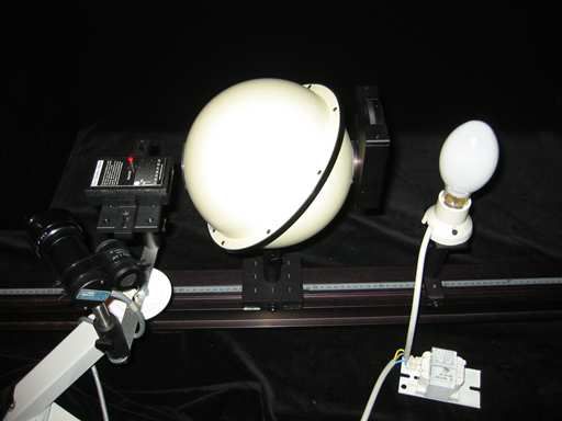
1Fig. 1.— Measurement of the acceptance angle.
Residual background ambience light could con-
taminate some data and the sensitivity of the re- Fig. 2.— Angular response of SQM in magnitudes.
sponse calibration equipment is low under 400 nm. Angles are positive downward and rightward.
2. Acceptance angle to Frequency Converter. The larger attenuation
of light incident on the filter with increasing an-
I checked the acceptance angle of the SQM se- gle makes the SQM angular response slightly nar-
rial n.0115 v.1.09 mounting it, both in horizontal rower than the detector angular response at large
and vertical position, on a rotation table (accuracy angles. The Half Width Half Maximum (HWHM)
0.01 degrees) placed at 1.289 m from a circular is ∼42 degrees. A factor 10 attenuation of a point
aperture with diameter 3.2 mm in front of LPLAB source is reached after 55 degrees. Optical inspec-
Spectral Radiance Standard (lamp 7) powered by tion shows that screening of the detector begins at
the LCRT-2000 radiometric power supply (radi- about 60-65 degrees.
ance stability 1% at 550 nm)(Cinzano 2003c, e). When comparing SQM measurements with
The set up is shown in fig. 1. Room temperature measurements taken with small field photome-
was maintained at 24.5±0.5 C. Background light ters it should be taken into account that night sky
has been subtracted. brightness is not constant with zenith distance. In
The readings of the instrument at each angle particular, artificial night sky brightness usually
are shown in fig. 2 in magnitude scale with arbi- grows with zenith distance with large gradients.
trary zero point. Open squares are data along the The brightness measured pointing the SQM to-
vertical plane, filled squares are data along the ward the zenith will be the weighted average of
horizontal plane. Angles are positive below the brightness down to a zenith distance of 60 degrees,
middle plane and at right, like in the data tables and then it will be greater (lower magnitude per
of the detector manufacturer (TAOS 2004). square second of arc) than the punctual zenith
Fig. 3 shows the same readings in a linear scale brightness:
normalized to its maximum. The figure also shows R 2π R π/2
the normalized output frequency of the detector I(θ, φ)D(θ) sin θ dθ dφ
I = 0 R 2π 0
R π/2 , (1)
at each angle provided by the detector manufac- D(θ) sin θ dθ dφ
0 0
turer (vertical is dashed, horizontal is dot-dashed).
This quantity is proportional to the measured ir- where I is the measured average radiance, D(θ) is
radiance because the detector is a Light Intensity the angular response given in fig. 3 and I(θ, φ)
21
0.8
weight function
0.6
0.4
0.2
10 20 30 40 50 60
zenith distance - degrees
Fig. 4.— Weight of the radiance at each angle of
incidence in the measured average radiance.
0
-0.1
mag arcsec^2
Fig. 3.— Angular response of SQM in a linear
scale. Lines show the normalized output frequency -0.2
of the detector at each angle provided by the de-
tector manufacturer, along the vertical (dashed)
-0.3
and horizontal (dot-dashed) planes.
Db
-0.4
is the radiance of the night sky in the field of
view of the SQM. Fig. 4 shows the weight func-
tion D(θ) sin θ for each angle of incidence θ. It is 5 10 15 20 25 30
peaked at about 30 degrees because going from 0 zenith distance deg
to π/2 the angular response decrease and the inte-
gration area grows. The effect is still more impor- Fig. 5.— Difference between SQM average and
tant when pointing the SQM to zenith distances of punctual brightness for a typical polluted site.
about 30 degrees because the instrument will col-
lect light from the zenith area down to the horizon.
3. Linearity
As an example, fig. 5 shows an estimate of the dif-
ference Db between the SQM average brightness I checked the linearity of our SQM analyzing
and the punctual brightness at each zenith dis- the residuals of a comparison with the IL1700 Re-
tance, based on a typical brightness versus zenith search Radiometer over the LPLAB Variable Low-
distance relationship at a polluted site measured light Calibration Standard (Cinzano 2003c). Data
by Favero et al. 2000 (in Cinzano 2000, fig.14) in are shown in figure 6.
Padova. It shows that at 30 degrees of zenith dis- The standard error is 2σ = ±0.028 mag
tance the SQM average brightness is brighter than arcsec−2 corresponding to 2.6%. Linear regres-
the punctual brightness of -0.4 mag/arcsec2 . Mea- sion has coefficient 0.0005. The uncertainty of the
surements beyond 30-45 degrees of zenith distance SQM due to deviations from linearity over a range
(i.e. under an elevation of 60-45 degrees) should of 12 magnitudes is likely smaller than 2.6%, be-
be avoided if the contamination by light sources cause measurements are affected by the stability
and by the luminous or dark landscape under the of the standard source (1%), the linearity of the
horizon cannot be checked. reference radiometer (1%) and the fluctuations of
31
Energy Response and QE
0.8
0.6
0.4
0.2
400 600 800 1000
wavelength nm
Fig. 7.— Normalized photodiode spectral respon-
sivity (solid line) and quantum efficiency (dashed
line).
Fig. 6.— Residuals of the comparison of the SQM
with a reference radiometer over a variable low-
light calibration standard. They give an upper 65-A radiometric power supply (source stability
limit to linearity. ±0.05%), a collector lens which collect the light
on the entrance slit of a Fastie-Ebert monocroma-
tor (wavelength accuracy ± 0.2%). A camera lens
the subtracted background. I did not check effects
focuses on the detectors the light coming from
of temperature on linearity but according to the
the output slit. At the moment at LPLAB we
manufacturer the detector is temperature com-
are mainly interested in checking the spectral re-
pensated for the ultraviolet-to-visible range from
sponse of our instruments rather than to obtain
320 nm to 700 nm (TAOS 2004).
accurate responsivity calibrations, so we use a ref-
erence detector with known response rather than
4. Spectral response
a certified spectral responsivity standard. The
I obtained the response curve of our SQM mul- reference detector was a Macam SD222-33 silicon
tiplying the spectral responsivity of the TAOS photodiode. Background stray light has been sub-
TSL237 photodiode by the transmittance of the tracted. Room temperature was maintained at
Hoya CM-500 filter, both provided by manufac- 23±0.5 C.
turers, and renormalizing to the maximum value. Fig. 9 shows the measured responsivity of the
Fig. 7 shows the normalized photodiode spectral SQM (squares) compared with its calculated re-
responsivity (solid line) and quantum efficiency sponsivity (line). The measurements follow the
(dashed line). The responsivity (response per unit calculated responsivity quite well. The reason of
energy) is not flat like the quantum efficiency (re- the difference over 550 nm is unknown, but main
sponse per photon) because photons at smaller factors could be an inclination of the filter in re-
wavelength have more energy. Fig. 8 shows the spect to the incoming light, a different laboratory
SQM normalized spectral responsivity (solid line), temperature, an uncertainty in the reference ra-
its normalized quantum efficiency and the Hoya diometer responsivity. Due mainly to light absorp-
filter transmittance (dotted line). tion from collector and camera lenses, the specific
I checked the calculated SQM responsivity with irradiance produced on the detector from the Low
LPLAB’s Low-Light-Level Spectral Responsiv- Light Level Responsivity Calibration Standard be-
ity Calibration Standard (Cinzano 2003c). The come low under about 400 nm, as shown in fig. 10.
equipment is composed by a standard lamp (lamp As a consequence, measurement errors due to the
3) powered by an high-accuracy Optronic OL- residual background stray light become large at
4response, QE, transmittance
100
80
60
40
20
400 500 600 700 800
wavelength nm
Fig. 8.— SQM normalized spectral responsivity
(solid line), quantum efficiency (dashed line) and
filter transmittance (dotted line). Fig. 9.— Measured SQM responsivity (squares)
and calculated SQM responsivity (line).
these wavelengths.
I checked changes in SQM spectral responsivity
due to the inclination of the incoming rays in re-
spect to the normal to the filter. For inclined rays
with off-normal angle of incidence θ, the normal-
ized filter transmittance is:
Tλ = (Tλ,⊥ )tθ /t⊥ , (2)
where tθ is the effective filter thickness:
1
tθ = q t⊥ . (3)
sin2 θ
1− n2
I assumed the index of refraction of the glass
n=1.55. The Full Width Half Maximum (FWHM)
of the normalized transmittance Tλ (θ) decreases
with the angle of incidence and, consequently, the
same behavior is followed by the normalized spec- Fig. 10.— Response of the LPLAB’s Low-Light-
tral responsivity Rλ (θ) = Sλ Tλ (θ), where Sλ is Level Spectral Responsivity Calibration Standard.
the photodiode response. Due to the large field
of view, the SQM collects light rays with a wide
range of incidence angles. The effective spectral
responsivity Rλ is the average of the spectral re-
sponsivity for each incidence angle Rλ (θ) weighted
by the angular response D(θ) given in fig.3 and by
the angular distribution of the spectral radiance
of the night sky in the field of view Iλ (θ, φ):
R 2π R π2
Rλ (θ)Iλ (θ, φ)D(θ) sin θ dθ dφ
Rλ = 0 R 2π 0
R π2 . (4)
0 0
Iλ (θ, φ)D(θ) sin θ dθ dφ
5100
1
normalized response
80
0.8
response
60
0.6
40
0.4
20
0.2
550 600 650 700
wavelength nm
400 500 600 700
Fig. 11.— Average spectral responsivity of the wavelength nm
SQM for an uniform night sky brightness (dashed
line), for light rays with 30 degrees incidence angle Fig. 12.— SQM normalized response (dotted
(dotted line) and for normal incidence (solid line) line), standard normalized responses of Johnson’s
B band, CIE scotopic, Johnson’s V band and
CIE photopic (dashed lines from left to right) and
Fig. 11 shows the average responsivity of the
emission spectra of an HPL mercury vapour lamp
SQM for an uniform night sky brightness (dashed
(solid line).
line), for rays with 30 degrees incidence angle (dot-
ted line) and for normal incidence (solid line). The
SQM could slightly underestimate the brightness scotopic and photopic eye responses. Its large
of the sky when it is polluted from sources with range recall the sensitivity of panchromatic films.
primary emission lines in correspondence of the These differences cannot be easily corrected with
right wing of the spectral responsivity, where the simple color corrections like in stellar photometry,
response is lower. However usual nighttime light- where sources have nearly blackbody spectra. In
ing lamps distribute their energy on many lines, facts, spectra of artificial night sky brightness typ-
apart from Low Pressure Sodium (LPS) lamps ically have strong emission lines or bands, so small
which, anyway, emit near the maximum of SQM differences in the wings of the response curve can
response. produce large errors.
In order to avoid mistakes, it is more correct
5. Relationship between SQM photomet- considering the SQM response as a new photo-
ric band and V-band metric system. It adds to the 226 known astro-
Fig. 12 shows for comparison the SQM nor- nomical photometrical systems listed in the Asiago
malized response (dotted line) and the standard Database on Photometric Systems (ADPS)(Moro
normalized responses of Johnson’s B band, CIE & Munari 2000, Fiorucci & Munari 2003). The
scotopic, Johnson’s V band and CIE photopic conversion factors between SQM photometric sys-
(dashed lines from left to right). These are some tem and other photometrical systems can be ob-
of the main photometric bands used in light pollu- tained based on the kind of spectra of the observed
tion photometry. The emission spectra of an HPL object. Hereafter I will call ”SQM” the brightness
mercury vapour lamp (solid line) is also shown. in mag arcsec−2 measured in the SQM passband.
Fig. 13 shows the same responses and the spectra The conversion between an instrument response
of an HPS High Pressure Sodium lamp (solid line). and a given standard response can be made multi-
It is evident that the SQM response is quite differ- plying the instrumental measurement by the con-
ent from these standard responses. SQM response version factor FC between the light fluxes collected
is also quite different from the old-time visual and by the standard response and by the instrumental
photovisual bands and from the combination of
61
normalized response
0.8
0.6
0.4
0.2
400 500 600 700
wavelength nm
Fig. 13.— SQM normalized response (dotted Fig. 14.— Conversion factors from SQM response
line), standard normalized responses of Johnson’s to Johnson’s V band.
B band, CIE scotopic, Johnson’s V band and CIE
photopic (dashed lines from left to right) and emis- lamps (Cinzano 2004), (v) the CIE Illuminant A
sion spectra of an HPS High Pressure Sodium (Planckian radiation at 2856 K), (vi) spectra of
lamp (solid line). HPS lamp and HPL lamp taken with WASBAM
(Cinzano 2002) and (vii) a series of blackbody
response: spectra at various temperatures. I adopted as
the standard response curve of Johnson’s (1953)
R R
fλ Rλ dλ f S dλ BV bands those given by Bessel (1990, tab. 2), a
FC = R R st,λ λ , (5) slightly modified version of the responses given by
fst,λ Rλ dλ fλ Sλ dλ
Azusienis & Straizys (1969).
where fλ is the spectral distribution of the ob- The conversion factors from SQM response to
served object, Rλ is the considered standard re- Johnson’s V band in magnitudes are shown in fig.
sponse, Sλ is the instrumental response and fst,λ 14 (see also tab. 2, column 1):
is the spectral distribution of the primary stan-
dard source for calibration, e.g. an A0V star for SQM − V = −2.5 log10 FC (7)
the UBV photometric system or Illuminant A for Here I will continue to call them conversion ”fac-
the CIE photometric system. The error due to an tors” even if SQM-V is an addictive constant. I
uncorrected spectral mismatch is: assumed here that both bands are calibrated over
1 − FC a primary standard AOV star spectra like alpha
ε= . (6) Lyrae. As absolute calibrated spectrum I adopted
FC
a synthetic spectrum of alpha Lyrae from Kurucz
I computed the conversion factors FC between scaled to the flux density of alpha Lyrae at 555.6
SQM response and V band response for: (i) a nm given by Megessier (1995), as discussed in de-
flat spectrum, (ii) an average moon spectrum ob- tail by Cinzano (2004).
tained assuming the lunar reflectance as given by The conversion factors are large, as expected
the Apollo 16 soil and a solar spectral irradiance because of the large difference in the response
spectrum from the WCRP model (see Cinzano curves. However, given that the SQM will be used
2004 for details), (iii) a natural night sky spectrum to measure light pollution and it will never be used
from Patat (2003) kindly provided by the author, to measure stars or sources with flat spectra, the
(iv) an averagely polluted sky spectrum obtained conversion factors for interesting sources lie in the
with a mix of spectra of natural night sky, High narrower range 0.35-0.6 mag arcsec−2 . They can
Pressure Sodium (HPS) lamps and HPL Mercury be reduced using a calibration source inside the
7Fig. 15.— SQM-V measured ¥ and calculated ¤. Fig. 17.— Limited range of interesting SQM-V.
Fig. 16.— SQM-V versus B-V is not linear. Fig. 18.— SQM-V for blackbodies (solid line).
same range, like Illuminant A or another lamp 15 shows the measured (filled squares) and calcu-
for nighttime lighting. As an example, referring lated (open squares) conversion factors from SQM
them to an Illuminant A lamp (SQM-V=0.48 mag response to the V band in magnitudes per square
arcsec−2 ) these conversion factors would lie in the arcsec in function of the B-V color index of the
range ±0.12 mag arcsec−2 . In fact Unihedron uses source. I shifted the zero-point of calculated fac-
for calibration a fluorescent lamp (their zero point tors to approximately fit the corresponding mea-
will be discussed later). The argument is further sured ones. Fig. 16 shows that the sources do not
faced in the following discussion. follow a simple B-V relation, as expected. Even
I measured the SQM-V conversion factors for if a polynomial (dashed line) could give a very
a number of sources by comparing SQM measure- rough fit to datapoints, a SQM-V versus B-V re-
ments with V-band measurements made with the lation does not make sense because data points
IL1700 research radiometer (accuracy of V band depend on the spectra of the source which in gen-
calibration ±4.9%, linearity 1%). Fig. 19 shows eral is not univocally determined by the color in-
the equipment used for some measurements. Fig. dex. Except few cases, lamps for nighttime light-
8ing are discharge lamps or LEDs, which are very
different from blackbodies. Fig. 17 shows that
if we consider only sources related to light pol-
lution, conversion factors lie in the range 0-0.25
mag arcsec−2 . As already pointed out, using an
higher zero-point or using an Illuminant A calibra-
tion source, the range could be restricted to about
±0.12 mag arcsec−2 .
Fig. 18 shows the SQM-V versus B-V relation-
ship for blackbodies (solid line). As expected, it
fits Illuminant A, the Moon, a flat spectra and al-
pha lyrae. The last is not fitted well because a
A0V star spectra it is not a true blackbody due to
absorption lines and bands. A polynomial interpo-
lation gives SQM−V = −0.162(B−V )2 +0.599(B−
V ) − 0.426. Linear regression gives SQM − V ≈
0.25(B −V )−0.26 when based on datapoints reg- Fig. 19.— The Variable Low Light Level Calibra-
ularly distributed within 0.4 ≤ B − V ≤ 1.7 and tion Standard. From left to right are visible the
SQM −V ≈ 0.28(B−V )−0.30 when based on dat- SQM and the reference detector, the Uniform In-
apoints within 0.5 ≤ B − V ≤ 1.7. tegrating Sphere, the aperture wheel and a test
lamp for road lighting (baffles removed). Spec-
Two independent authors tested the SQM at
tral irradiance/radiance standard lamps with ra-
the telescope over standard stars finding a good
diometric power supplies and optical devices are
agreement with SQM − V 0 ≈ 0.2(B 0 − V 0 ) (Uni-
used in other configurations.
hedron, priv. comm.). The smaller angular co-
efficient could be explained by the differences be-
tween stellar and blackbody spectra, i.e. by the sources related to light pollution would have been
different distribution of stellar datapoints in re- reduced to the range ≈ ±0.12 mag arcsec−2 . My
spect to blackbody datapoints on the plane SQM- best calibration to Illuminant A, obtained with
V versus B-V. The different zero point is likely due the LPLAB Low Light Level Calibration Stan-
to the fact that the relation has been obtained dard, the spectral radiance standard lamp no. 7
with outside-the-atmosphere magnitudes V’ and powered by the LCRT-2000 radiometric power
B’. As an example, assuming an extinction of 0.35 supply (radiance stability 1% at 550 nm) and
mag in V and 0.15 mag in B and replacing V’=V- the IL1700 reference radiometer (accuracy of V
0.35 and B’=B-0.15, where V and B are the ap- band calibration ±4.9%, linearity 1%), provides
parent magnitude below the atmosphere, we ob- V = SQM − 0, 108 ± 0.054 mag arcsec−2 . The er-
tain SQM − V = 0.2(B − V ) − 0.31 in agree- rorbar includes both the measurement uncertainty
ment with my previous results. The zero point and the V band calibration uncertainty of the ref-
of the current SQM calibration made by Unihe- erence photometer. The condition SQMnew =V
dron gives SQM≈V’ for stars with B’=V’, above for Illuminant A is satisfied increasing the current
the atmosphere, and consequently the below-the- SQM zero point of 0.108 mag arcsec−2 or sub-
atmosphere SQM-V correction factor for the alpha tracting this number from current measurements.
Lyrae spectrum come out different from zero. Fig. Given the many uncertainty factors playing when
18 shows that for alpha Lyr is SQM-V=-0.35 mag comparing instruments, before an official change
arcsec−2 . of zero point a wider comparison should be car-
Given that the instrument is not used for mea- ried, better if also including measurements over
surements of stars at the telescope, this feature the night sky. The SQM-V conversion factors af-
appears not necessary. On the contrary, by re- ter the adjustment are listed here:
ferring the calibration to an Illuminant A and
the zero point to the condition SQM=V (below
the atmosphere), the conversion factors for the
96. Addition of filters for CIE photopic,
CIE scotopic, V-band, B-band
I also calculated with eq. 5 the spectral mis-
match correction factors between SQM response
and the CIE photopic, CIE scotopic, V-band, B-
band responses, when specific filters are added. I
considered addition of filters rather than replace-
ment of the existing filter because more on line
with the SQM philosophy of simple and fast mea-
surements. Anyone can add a filter in front of the
instrument whereas replacement requires specific
work. Calculations assume that the instrument is
properly calibrated over an Illuminant A for the
CIE photometric system and over an AOV star,
like alpha Lyrae, for Johnson’s B and V (or prop-
erly rescaled to it). I choose for these tests an
Optec Bessell V filter, an Optec Bessell B filter,
Fig. 20.— SQM-V conversion factor (mag an Oriel G28V photopic filter and a scotopic fil-
arcsec−2 ) for a night sky model spectrum, in func- ter.
tion of its V brightness and B-V color index. Fig. 21 shows the standard response (solid line)
and the SQM+filter response (dashed line) for CIE
source SQM-V photopic (top) and CIE scotopic responses (bot-
HPS lamp +0.11 tom). The SQM response is also shown for com-
HPL lamp +0.00 parison (dotted line). The spectral mismatch cor-
illuminant A +0.00 rection factors for the photopic and scotopic re-
sky natural +0.06 sponses are presented in tab. 1. The standard re-
sky polluted +0.08 sponses of the CIE photometric system are given
moon ab. atm. -0.13 in CIE DS010.2/E where they are called ”spectral
luminosity efficiency functions”. The instrument
I finally explored the relation between the con-
is assumed to have been calibrated over an Illumi-
version factor SQM-V for the night sky spectrum
nant A spectrum. Tab. 1 shows that after the ap-
and its V brightness and B-V color index. Follow-
plication of the filter the spectral mismatch correc-
ing Cinzano (2004), I constructed a very simple
tion factors became quite small, so that correction
model spectra for polluted sky assuming that the
could be neglected. The match to the CIE pho-
night sky brightness spectrum fsky is given by the
topic response could be further improved choosing
sum of a natural night sky spectrum, an HPS lamp
a filter with the left wing at larger wavelengths.
spectrum and an HPL mercury vapour lamp spec-
The match of scotopic response is adequate.
trum, each of them multiplied by a coefficient kn ,
independent by the wavelength: Fig. 22 shows the standard response (solid line)
and the SQM+filter response (dashed line) for V
fsky = fnat + k1 (k2 fHP S + (1 − k2 )fHP L ) (8) band (top) and B band (bottom). The SQM re-
sponse is also shown for comparison (dotted line).
With this spectrum I calculated the function The spectral mismatch correction factors in mag-
SQM − V (Vsky , (B − V )sky ). Fig. 20 shows the nitudes per square arcsec for the Johnson’s B and
conversion factor SQM-V of the night sky in mag- V bands are presented in tab. 2. The instrument
nitudes per square arc second in function of the V is assumed to have been calibrated over an AOV
brightness and the B-V color index. The conver- star spectra, like alpha Lyrae, or properly rescaled
sion factor is referred to the natural sky, i.e. its to it. The match of V band response is adequate.
adds to the SQM-V of the natural sky (+0.48 mag The match to the B band could be further im-
arcsec−2 if calibration refers to alpha Lyr or +0.06 proved choosing a filter with the left wing at lower
mag arcsec−2 if calibration refers to Illuminant A).
101 1
normalized response
normalized response
0.8 0.8
0.6 0.6
0.4 0.4
0.2 0.2
400 450 500 550 600 650 700 750 450 500 550 600 650 700
wavelength nm wavelength nm
1
1
normalized response
normalized response
0.8
0.8
0.6
0.6
0.4
0.4
0.2 0.2
0
400 450 500 550 600 650 375 400 425 450 475 500 525 550
wavelength nm wavelength nm
Fig. 21.— Top panel: CIE photopic response Fig. 22.— Top panel: V band response (solid line)
(solid line) and SQM + G28V filter (dashed line). and the SQM+ Optec V filter (dashed line). Bot-
Bottom panel: CIE scotopic response (solid line) tom panel: B band response (solid line) and the
and SQM + scotopic filter (dashed line). SQM+ Optec B filter (dashed line).
wavelengths. calibration factor and extinction are properly eval-
uated with the Bouguer method but are wrongly
7. Further notes on measurement compar- given as ”above the atmosphere” when counts
ison from standard stars and sky background are com-
pared without accounting for extinction from the
When comparing SQM measurements with top of the atmosphere to the ground.
measurements made with other instruments, it b) SQM includes all stars whereas measurements
should be taken also into account that: of sky background made with telescopes usually
a) SQM, like the other photometers, radiome- exclude field stars more luminous than a given
ters, luminancemeters and WASBAM, correctly magnitude. When the artificial brightness is not
measures the night sky brightness ”below the at- predominant, the contribution of these stars to
mosphere”, the way it was. On the contrary, the night sky brightness should be added before
measurements made with instruments applied to comparing telescopical measurements with SQM
telescopes are ”below the atmosphere” when the measurements (table 3.1 of Cinzano 1997 could be
11source Photopic Scotopic a) conversion factors from SQM photometric sys-
no filter filter no filter filter tem to Johnson’s V band are in the range 0-0.25
HPS lamp 0,78 1,01 1,70 1,00 mag arcsec−2 when considering only main sources
HPL lamp 1,02 1,06 1,22 1,06 of interest for light pollution. They are presented
illuminant A 1,00 1,00 1,00 1,00 in fig. 15.
sky natural 0,96 1,05 0,79 1,02 b) conversion factors for the polluted sky differs
sky polluted 0,85 1,02 1,37 1,02 from the factor for the natural sky less than ±0.05
moon ab. atm. 1,20 1,08 0,79 1,02 mag arcsec−2 and can be related to the sky V
flat 1,35 1,08 0,84 1,03 brightness and B-V color index (fig. 20).
c) quick conversion factors to obtain V band
Table 1: Spectral mismatch correction factors for brightness from SQM measured brightness with
CIE photopic and scotopic responses. current factory calibration are proposed here be-
low for further testing. They are chosen to mini-
source V band B band
mize the expected uncertainty ∆V .
no filter filter no filter filter
HPS lamp +0,59 -0,05 -2,26 +0,10 Conversion for V ∆V
HPL lamp +0,48 +0,04 -0,63 -0,01
Natural & polluted sky SQM-0.17 ±0.07
illuminant A +0,48 +0,04 -1,37 +0,20
Lamps, sky, moonlight SQM-0.11 ±0.14
sky natural +0,54 +0,02 -0,57 +0,04
sky polluted +0,56 -0,02 -1,34 +0,03 First line is for typical natural or polluted sky,
moon ab. atm. +0,35 +0,01 -0,59 +0,07 the second line is for surfaces lighted by artificial
flat +0,23 +0,01 -0,43 +0,02 sources (HPS, HPL, Illuminant A), natural night
alpha Lyrae +0,00 +0,00 +0,00 +0,00 sky, polluted night sky or moonlight. The uncer-
tainty of the V band calibration of the reference
Table 2: Spectral mismatch correction factors for photometer used in test measurements is included
V and B responses in magnitude per square arcsec. in ∆V . Units are V mag/arcsec2 .
d) SQM gives the average night sky brightness,
weighted for the angular response inside an ac-
used). When the night sky brightness is referred
ceptance area which has a diameter of 55 degrees
to naked eye, only stars to magnitude 6 should be
down to 1/10 attenuation. Due to the gradients
included. However the contribution of stars more
of the night sky brightness with zenith distance,
luminous of mag 5 (included) is only 6% of the
the SQM average brightness is larger (smaller mag
natural night sky brightness.
arcsec−2 ) than the brightness measured by a nar-
row field photometer pointed in the same direc-
8. Conclusions
tion, as shown e.g. in fig. 5. In order to roughly
Sky Quality Meter is a fine and interesting estimate the punctual V band brightness, add to
night sky brightness photometer. Its low cost and SQM measurements 0 to 0.3 mag/arcsec2 at zenith
pocket size allow to the general public to quan- or 0 to 0.4 mag/arcsec2 at 30 degrees of zenith dis-
tify the quality of the night sky. In order to un- tance, depending on the pollution level.
derstand the measurements made by it, I checked e) SQM correctly gives the brightness ”below the
acceptance angle, linearity and spectral responsiv- atmosphere” whereas telescopical measurements
ity. I analyzed the conversion between SQM pho- calibrated on standard stars give ”below the at-
tometric system and Johnson’s B and V bands, mosphere” brightness only when the extinction is
CIE photopic and CIE scotopic responses and de- properly evaluated and accounted for.
termined for some typical spectra both the conver- f) SQM correctly fully includes the stellar compo-
sion factors and the spectral mismatch correction nent in the measured brightness whereas telescop-
factors when specific filters are added. ical measurements frequently exclude stars more
luminous than a given magnitude.
Comparing SQM measurements with measure-
g) addition of commercial Johnson’s B band, V
ments taken with other instruments it should be
band, CIE photopic or CIE scotopic filters in
taken into account that:
front of the SQM with proper calibrations, makes
12the spectral mismatch correction factors very low. Cinzano, P. 2003e, The ISTIL/LPLAB Irradiance
This allows reasonably accurate multiband mea- and Radiance Standard, ISTIL Int. Rep. 6,
surements, including B-V color indexes and sco- Thiene, Italy
topic to photopic ratios.
Cinzano, P. 2004, in prep.
Cinzano, P., Falchi F. 2003, Mem. Soc. Astron. It.,
ACKNOWLEDGMENTS 74, 458-459
Fiorucci, F., Munari U. 2003, A&A, 401, 781-796
LPLAB was set up as part of the ISTIL project
‘Global monitoring of light pollution and night Hoya 2004, www.newportglass.com/hcm500.htm
sky brightness from satellite measurements’ sup-
ported by ASI (I/R/160/02). Some instrumen- Johnson H.L., Morgan W.W. 1953, ApJ 117, 313
tation has been funded by the author, the Inter-
Megessier, C. 1995, A&A, 296, 771-778
national Dark-Sky Association, Tucson, the BAA
Campaign for Dark-Sky, London, the Associazione Moro N., Munari U. 2000, A&AS, 147, 361-628 on-
Friulana di Astronomia e Metereologia, Remanza- line at http://ulisse.pd.astro.it/Astro/ADPS/
cco and Auriga srl, Milano.
Patat, F. 2003, A&A, 400, 1183-1198
REFERENCES
TAOS 2004, TSL237 High-Sensivity Light-to-
Azusienis A. & Straizys V. 1969, Soviet Astron., Frequancy Converter, www.taosinc.com
13, 316
Bessel, 1990, PASP, 102, 1181-1199
CIE 2001, The CIE System of Physical Photome-
try, Draft Standard 010.2/E
Cinzano, P. 1997 Inquinamento luminoso e pro-
tezione del cielo notturno, Istituto Veneto di
Scienze Lettere ed Arti, Venezia, on-line at
http://dipastro.pd.astro.it/cinzano/
Cinzano, P. 2000, Mem. Soc. Astron. It., 1, 113-
130
Cinzano, P. 2003a, A laboratory for the photom-
etry and radiometry of light pollution, poster,
meeting IAU Comm. 50 Working Group ”Light
Pollution”, XXV General Assembly, Sidney 25
June - 2 July 2003
Cinzano, P. 2003b, Mem. Soc. Astron. It. Suppl.,
3, 414-318
Cinzano, P. 2003c, The Laboratory of Photometry
and Radiometry of Light Pollution (LPLAB),
ISTIL Int. Rep. 7, Thiene, Italy, www.lplab.it
Cinzano, P. 2003d, Characterization of the Vari-
able Low Light Level calibration Standard, IS-
TIL Int. Rep. 3, Thiene, Italy
This 2-column preprint was prepared with the AAS LATEX
macros v5.2.
130 ISTILInternal Report
c 2005 ISTIL, Thiene
°
www.istil.it
www.lplab.it
14You can also read