Short-term forecasting COVID-19 cumulative confirmed cases: Perspectives for Brazil - arXiv
←
→
Page content transcription
If your browser does not render page correctly, please read the page content below
Short-term forecasting COVID-19 cumulative confirmed cases:
                                                                        Perspectives for Brazil
                                                     Matheus Henrique Dal Molin Ribeiroa,b,∗, Ramon Gomes da Silvaa , Viviana Cocco
                                                                       Marianic,d , Leandro dos Santos Coelhoa,d
                                            a
                                              Industrial & Systems Engineering Graduate Program (PPGEPS), Pontifical Catholic University of Parana
                                                            (PUCPR). 1155, Rua Imaculada Conceicao, Curitiba, PR, Brazil. 80215-901
                                            b
                                              Department of Mathematics, Federal Technological University of Parana (UTFPR). Via do Conhecimento,
                                                                        KM 01 - Fraron, Pato Branco, PR, Brazil. 85503–390
arXiv:2007.12261v1 [q-bio.PE] 21 Jul 2020

                                                   c
                                                     Mechanical Engineering Graduate Program (PPGEM), Pontifical Catholic University of Parana
                                                            (PUCPR). 1155, Rua Imaculada Conceicao, Curitiba, PR, Brazil. 80215-901
                                                d
                                                  Department of Electrical Engineering, Federal University of Parana (UFPR). 100, Avenida Coronel
                                                                   Francisco Heraclito dos Santos, Curitiba, PR, Brazil. 81530-000

                                            Abstract
                                            The new Coronavirus (COVID-19) is an emerging disease responsible for infecting millions of
                                            people since the first notification until nowadays. Developing efficient short-term forecasting
                                            models allow knowing the number of future cases. In this context, it is possible to develop
                                            strategic planning in the public health system to avoid deaths. In this paper, autoregressive
                                            integrated moving average (ARIMA), cubist (CUBIST), random forest (RF), ridge regression
                                            (RIDGE), support vector regression (SVR), and stacking-ensemble learning are evaluated
                                            in the task of time series forecasting with one, three, and six-days ahead the COVID-19
                                            cumulative confirmed cases in ten Brazilian states with a high daily incidence. In the stacking
                                            learning approach, the cubist, RF, RIDGE, and SVR models are adopted as base-learners
                                            and Gaussian process (GP) as meta-learner. The models’ effectiveness is evaluated based
                                            on the improvement index, mean absolute error, and symmetric mean absolute percentage
                                            error criteria. In most of the cases, the SVR and stacking ensemble learning reach a better
                                            performance regarding adopted criteria than compared models. In general, the developed
                                            models can generate accurate forecasting, achieving errors in a range of 0.87% - 3.51%,
                                            1.02% - 5.63%, and 0.95% - 6.90% in one, three, and six-days-ahead, respectively. The
                                            ranking of models in all scenarios is SVR, stacking ensemble learning, ARIMA, CUBIST,
                                            RIDGE, and RF models. The use of evaluated models is recommended to forecasting and
                                            monitor the ongoing growth of COVID-19 cases, once these models can assist the managers
                                            in the decision-making support systems.
                                            Keywords: ARIMA, COVID-19, Forecasting, Decision-making, Machine learning,
                                            Time-series

                                                ∗
                                                    Corresponding author
                                                    Email address: matheus.dalmolinribeiro@gmail.com (Matheus Henrique Dal Molin Ribeiro)

                                            Preprint submitted to Chaos, Solitons & Fractals                                         July 27, 2020
1. Introduction
The new Coronavirus (COVID-19) is an emerging disease responsible for infecting mil-
lions of people and killing thousands worldwide since the first notification until nowadays,
according to the World Health Organization (WHO) [1, 2]. Also according to WHO, Brazil
registered 40.581 confirmed cases until April 22th 2020, holding the 12th position in the world
ranking in the number of confirmed cases of COVID-19, and 2nd position in the Americas
(behind the United States of America).
Due to the impacts of the COVID-19 pandemic in people’s lives and the world’s economy,
the governments and population are most concerned with (i) when the COVID-19 outbreak
will peak; (ii) how long the outbreak will last and (iii) how many people will eventually be
infected [3]. Further, Boccaletti et al. [4] have identified at least three scientific communities
that may cooperate in the effort to deal with the current pandemic: (i) the community of
applied mathematicians, virologists and epidemiologists, developing sophisticated diffusion
models to the specific properties of a given pathogen; (ii) the community of complex systems
scientists who study the spread of infections using compartmental models, using methods
and principles from statistical mechanics and nonlinear dynamics; and (iii) the community
of scientists who incorporate artificial intelligence (AI) and most specifically deep learning
approaches to produce accurate predictive models. Also, different studies are evaluating the
impacts of COVID-19 on society, whether through predictions of future cases, as well as
variables capable of helping to understand the spread of this disease [5, 6, 7, 8, 9].
Moreover, epidemiological time series forecasting plays an important role in health public
system, once it allows the managers to develop strategic planning to avoid possible epidemics.
Forecasting diseases as accurate as possible is important due to their impact on the public
health system. To ensure this accuracy, AI models have been widely used to forecast epi-
demiological time series over the years [10, 11, 12]. Moreover, in the AI context, Vaishya et
al. [13] presented a review of trends in COVID-19 data analysis.
Regarding this context, the objective of this paper is to explore and compare the predic-
tive capacity of machine learning regression and statistical models, in the task of forecasting
one, three, and six-days-ahead COVID-19 cumulative cases in Brazil. In this respect, datasets
of ten Brazilian states some with a high incidence of COVID-19 until now, like Sao Paulo and
Rio de Janeiro, are adopted to evaluates the forecasting efficiency through of the autoregres-
sive integrated moving average (ARIMA), cubist regression (CUBIST), random forest (RF),
ridge regression (RIDGE), support vector regression (SVR), and stacking-ensemble learning
models. In the stacking learning modelling, which is an effective ensemble learning approach
[14, 15], CUBIST, RF, RIDGE, and SVR are used as base-learners (weak models), and Gaus-
sian process (GP) as meta-learner (strong model). The out-of-sample forecasting accuracy of
each model is compared by some performance metrics such as the improvement percentage
index (IP), mean absolute errors (MAE), and symmetric mean absolute percentage error
(sMAPE).
The contributions of this paper can be summarized as follows:
• The first contribution is related to the presentation of a novel analysis of the forecast
model for cumulative confirmed cases of COVID-19 in Brazil, whose accuracy of the
2models assists governors in decision-making to contain the pandemic and strategies
concerning the health system;
• The second contribution, we can highlight the use of heterogeneous machine learning
models, as well as the stacking-ensemble learning approach to forecast the Brazilian
cumulative confirmed cases of COVID-19;
• Also, this paper evaluates models forecasting in a multi-day-ahead forecasting strategy.
The forecasting time horizons are the interval of one, three, and six-days-ahead. This
range of the forecasting time horizon allows us to verify the effectiveness of the predict-
ing models in different scenarios, helping in future strategies in fighting COVID-19.
The remainder of this paper is organized as follows: Section 2.1 a brief description of the
dataset adopted in this paper is given. The forecasting models applied in this study are de-
scribed in Section 2.2. Section 3 details the procedures applied in the research methodology.
Results obtained and related discussion about models’ forecasting performance are given on
Section 4. Finally, Section 5 concludes this work with considerations and some directions for
future research proposals.
2. Material and Methods
This section presents the description of the material analyzed (Section 2.1) as well as the
models description applied in this paper (Section 2.2).
2.1. Dataset Description
The collected dataset refers to the cumulative confirmed cases of COVID-19 that occurred
in Brazil until April, 18 or 19 of 2020. The dataset was collected from an API [16] that
retrieves the daily information about COVID-19 cases from all 27 Brazilian State Health
Offices, gather them, and make it a publicly available. Among the 27 federative units (26
states and one federal district), ten states some with a high incidence of COVID-19 cases
and other states with lower temperatures, states from south of Brazil, were chosen, among
them are Amazonas (AM), Bahia (BA), Ceara (CE), Minas Gerais (MG), Parana (PR), Rio
de Janeiro (RJ), Rio Grande do Norte (RN), Rio Grande do Sul (RS), Santa Catarina (SC),
and Sao Paulo (SP). The measurement period of each state varies, once each state counts
since the day of its first case until the day of the last report. The cumulative confirmed cases
and deaths of each state, as well as the period from the first and last reports, are illustrated
in Table 1. The change in the way of accounting for the number of cases, by the health
departments, may change the data presented here.
3Table 1: First and last report dates by state
Number of Cumulative Cumulative
State First report Last report
observed days confirmed cases deaths
AM 34 13/03/2020 19/04/2020 2044 182
BA 43 06/03/2020 19/04/2020 1249 45
CE 35 16/03/2020 19/04/2020 3306 189
MG 42 08/03/2020 19/04/2020 1154 39
PR 36 12/03/2020 18/04/2020 960 49
RJ 38 05/03/2020 19/04/2020 4675 402
RN 30 12/03/2020 18/04/2020 561 26
RS 38 10/03/2020 19/04/2020 869 26
SC 39 12/03/2020 19/04/2020 1025 35
SP 53 25/02/2020 19/04/2020 14267 1015
A heatmap of the cumulative confirmed cases is presented in Figure 1.
AM CE
RN
Cumulative
confirmed cases
BA
10000
MG 5000
SP RJ
PR
SC
RS
Figure 1: Heatmap of the cumulative confirmed cases of the analyzed states
2.2. Methodologies
This section describes a brief of each model employed in the data analysis.
• ARIMA is a Box & Jenkins modelling usually employed to deal with non-stationary
time series. In fact, the ARIMA model is full specified by autoregressive (p), different
degrees of trend differences (d ), and moving average operators (q). These parameters
4are used do define the model order, and usually defined by grid-search, as well as
by autocorrelation and partial autocorrelation function. In this context, the model is
described as ARIMA(p,d,q) [17].
• CUBIST is a rule-based model, which performs predictions following the regression
of trees principle [18]. Through the use of a committee of the rules, and using the
neighborhood concept similar to k-nearest-neighbor modelling, the final forecasting is
obtained.
• GP is composed of a set of random variables Gaussian distributed and fully specified
by its mean and covariance (kernel) function [19]. In this paper, the GP with a linear
kernel is adopted.
• RIDGE is a regularized regression approach [20] which employs a penalization term in
the ordinary least squares algorithm. It is an effective tool, once it reduces the bias of
parameter estimates by controlling the standard errors. Moreover, the model can deal
with inputs multi-collinearity problem.
• RF is a bagging ensemble-based model, which combines the bagging advantages char-
acterized by the creation of multiple samples, with refitting through of the bootstrap
technique, from the same set of data, and random selection of predictors to compose
each node of the decision tree [21]. RF is a fast and robust supervised learning method
able to deal with the randomness of the time series. Furthermore, it is interesting
because, in addition to being an ensemble approach, only the number of predictors for
each node needs to be tuned.
• SVR consists in determining support vectors (points) close to a hyperplane that max-
imizes the margin between two-point classes obtained from the difference between the
target value and a threshold. To deal with non-linear problems SVR takes into ac-
count kernel functions, which calculates the similarity between two observations. In
this paper, the linear kernel is adopted. The main advantages of the use of SVR lies
in its capacity to capture the predictor non-linearity and then use it to improve the
forecasting cases. In the same direction, it is advantageous to employ this perspective
in this case study adopted, since that the samples are small [22].
• Stacked Generalization or stacking is an ensemble-based approach [23] which combines
through a meta-learner the predictions of a set of weak models (base-learners) to obtain
a stronger learner. This approach usually operates into two levels, where in the first
level the base-learners are trained and its predictions are obtained. In the next stage, a
meta-learner uses, as inputs, the predictions of the previous level in the training phase.
The stacking predictions are obtained from meta-learner. The main advantage of the
stacking ensemble is that this approach can improve the accuracy and additionally
reduce error variance [14].
53. Proposed forecasting framework
This section describes the main steps in the data analysis adopted by CUBIST, RF,
RIDGE, SVR, and stacking models. Also, the ARIMA modelling is described.
Step 1: Firstly, the raw data is split into training and test datasets. The test dataset
is composed of six last observations, and the training dataset by the remain samples [14].
The training data are centered by its mean value and divided by its standard deviation.
To develops multi-days-ahead COVID-19 cases forecasting, recursive strategy is employed
[24]. In this aspect, one model is fitted for one-day-ahead forecasting. Next, the recursive
strategy uses the forecasting value as an input for the same model to forecast the next step,
continuing this manner until reaching the desirable horizon. The training structure adopted
in this paper is stated as follows,
y(t+1) = f yt , . . . , yt+1−ny + ∼ N (0, σ 2 ),
(1)
in which f is a function related to the adopted model in the training stage, yt+1 is the
COVID-19 case one-day-ahead, ny = 5 are the past confirmed cases, is the random error,
following a normal distribution with zero mean and constant variance. In this paper, the aim
is to obtain the cases up to H next days, especially up to 1 (ODA, one-day-ahead), 3 (TDA,
three-days-ahead), and 6-days-ahead (SDA, six-days-ahead), respectively. The following
structures are considered,
f yt , yt−1 , . . . , yt , . . . , yt−ny +1
if h = 1
ŷt+h = f ŷt+h−1 , . . . , ŷt+h , . . . , yt , . . . , yt+h−ny if h ∈ [2, ny ] (2)
f ŷt+h−1 , . . . , ŷt+h−ny if h ∈ [ny + 1, . . . , H],
where ŷt+h is the forecast value at time t and forecast horizon up to h, yt+h−ny and ŷt+h−ny
are the previously observed and forecast cases lags in ny = 5 days. The ny value is chosen
through grid-search with purpose to capture the best data behavior.
Step 2: In the stacking modelling, the base-learners CUBIST, RF, RIDGE, SVR are
trained and its forecasting are used as inputs for meta-learner GP. In the training stage,
leave-one-out cross-validation with a time slice is adopted [14]. Finally, the out-of-sample
forecasts are computed. These approaches are developed using the caret package [25]. The
ARIMA modeling is performed through the use of forecast package [26, 27] with use of
auto.arima function. To define the ARIMA order, grid-search is adopted, and the most
suitable order is that reach a lower Akaike and Bayesian Akaike criteria information. Both
analyses are developed using R software [28]. All hyperparameters employed in this study
are presented in Table B.1 in Appendix B.
Step 3: To evaluate the effectiveness of adopted models, from obtained forecasts out-
of-sample (test set), performance IP (3), MAE (4), and sMAPE (5) criteria are computed
as
n
1X
MAE = |yi − ŷi | , (3)
n i=1
6n
1X ŷi − yi
sMAPE = , (4)
n i=1 (|yi | + |ŷi |/2)
Mc − Mb
IP = 100 × , (5)
Mc
where n is the number of observations, yi and ŷi are the i -th observed and predicted values,
respectively. Also, the Mc and Mb represent the performance measure of compared and best
models, respectively.
Figure 2 presents the proposed forecasting framework.
A COVID-19 CASES C STACKING FRAMEWORK
Raw data of each
Brazilian state
Split
Training set Test set
System Inputs and Outputs
Base-learners
Layer-0
CUBIST RF RIDGE SVR
B GENERAL APPROACHES Base-learners Predictions
Meta-learner
ARIMA
Layer-1
GP System Inputs
Meta-learner Prediction
RIDGE Stacking
Performance
metrics
CUBIST SVR MAE sMAPE IP
RF
Figure 2: Proposed forecasting framework
4. Results
This section describes the results of the developed experiments in forecasts out-of-sample
(test set). First, Section 4.1 compares the results of evaluated models over ten datasets and
three forecasting horizons adopted. In Table A.1 in Appendix A, the best results regarding
accuracy are presented in bold. Additionally, Figures 3 up to 4 illustrate the relation between
observed and predicted values achieved by models with best set of performance measures
depicted in Table A.1, as well as box-plots for out-of-sample errors are illustrated in Figure
5.
74.1. Performance Measures for compared models
In this section, the main results achieved by the best model regarding MAE and sMAPE
criteria are presented for short-term forecasting multi-days- ahead of cumulative cases of
COVID-19 from ten Brazilian states.
• AM: In this state, CUBIST, and RIDGE approaches could be considered to forecasting
COVID-19 cases. In fact, in respect to ODA and TDA, CUBIST outperforms models,
while for SDA the RIDGE achieves better accuracy regarding MAE and sMAPE than
others. The improvement in the MAE for ODA and TDA achieved by CUBIST ranges
between 6.58% - 92.77%, and 11.39% - 88.54%, respectively. Through sMAPE analysis,
the RIDGE model outperforms other models, and this criterion is reduced in the range
of 16.46% - 91.88%, for SDA horizon.
• BA, MG, RS, and SP: For these states, in all forecasting windows, the SVR approach
achieved better accuracy than other models, for both MAE and sMAPE criteria in the
multi-days-ahead forecasting task of the confirmed number of COVID-19. In fact, the
improvement in sMAPE is ranged in 13.26% - 95.11%, 4.23% - 94.88%, and 38.59%
- 95.24%, respectively, in ODA, TDA, and SDA forecasting horizons. Moreover, the
same behavior is observed when the improvement in sMAPE criterion is obtained.
• CE and RN: In the CE state, the ARIMA model has a better performance in the
forecasting out-of-sample than other models for ODA and TDA time windows. In this
aspect, for MAE criterion, the improvement is ranged between 72.36% - 98.03%, and
45.93% - 92.40%, for ODA, and TDA time windows, respectively. For sMAPE, the
improvement on ODA, and TDA horizons is 65.06% - 97.84%, and 32.81% - 92.53%,
respectively. The SVR has better results than ARIMA model for SDA. Considering the
RN state, the same analysis is developed for ODA, and TDA horizons. The exception
to the SDA horizon, in which the CUBIST model has better effectiveness in the MAE
and sMAPE criteria than remain models.
• PR, RJ, and SC: For these states localized into the south region (PR and SC) and
southeast region (RJ) of Brazil, the most appropriate approach to forecast cumula-
tive cases of COVID-19 is the stacking ensemble, exception in ODA horizon, when
ARIMA model has better results. Stacking overcomes the drawback of single models
and achieves the best accuracy than other models. In fact, for these states, the im-
provement in MAE and sMAPE are between 14.01% - 94.68%, and 17.48% - 95.41%,
respectively, for ODA horizon. The improvement in order forecasting horizons presents
the same behavior of ODA, with the greatest magnitude of improvement for TDA and
SDA.
Remark: In this experiment, 180 scenarios (10 datasets, 3 forecasting horizons, and
6 models) were evaluated for the task of forecasting cumulative COVID-19 cases. In an
overview, the best models for each state, obtained sMAPE ranged between 0.87% - 3.51%,
1.02% - 5.63%, and 0.95% - 6.90% for ODA, TDA, and SDA forecasting, respectively. The
8ranking of models in all scenarios is SVR, stacking ensemble, ARIMA, CUBIST, RIDGE,
and RF models. In contrast to finds of [29], for the datasets evaluated in this paper, ARIMA
modelling was effective in some situation for very-short horizons When the horizon is SDA,
ARIMA model has worst performance than most of compared models. However, for ODA
the applications are limited. From a broader perspective, the efficiency of SVR is due to its
ability to deal with small size dataset, while the stacking ensemble combines the advantages
of several single models to learn the data behavior and obtain forecasts similar to observed
values. On the other hand, the difficulty of the RF model to forecasting cumulative COVID-
19 cases could be attributed to the fact that this approach requires more observations to
effectively learn the data pattern.
Observed Observed
ODA-CUBIST ODA-ARIMA
1200
SDA-RIDGE SDA-SVR
2000
TDA-CUBIST TDA-SVR
Cumulative confirmed cases
Cumulative confirmed cases
1500
800
1000
400
500
Training Test Training Test
0
0
23/03 30/03 06/04 13/04 20/04 15/03 01/04 15/04
Date Date
(a) AM (b) BA
(c) CE (d) MG
Figure 3: Predicted versus observed cumulative confirmed cases of COVID-19 for AM, BA, CE, and MG
states
According to the information depicted in Figures 3 and 4 it is possible to identify that the
9(a) PR (b) RJ
Observed Observed
ODA-ARIMA ODA-SVR
SDA-CUBIST SDA-SVR
TDA-ARIMA TDA-SVR
Cumulative confirmed cases
Cumulative confirmed cases
750
400
500
200
250
Training Test Training Test
0
0
23/03 30/03 06/04 13/04 15/03 01/04 15/04
Date Date
(c) RN (d) RS
Observed Observed
15000
ODA-ARIMA ODA-SVR
SDA-Stacking SDA-SVR
TDA-Stacking TDA-SVR
Cumulative confirmed cases
Cumulative confirmed cases
900
10000
600
5000
300
Training Test Training Test
0
0
15/03 01/04 15/04 01/03 15/03 01/04 15/04
Date Date
(e) SC (f) SP
Figure 4: Predicted versus observed cumulative confirmed cases of COVID-19 for PR, RJ, RN, RS, SC, and
SP states
10behavior of the data is learned by the evaluated models, which can forecasting compatible
cases with the observed values. The good performance obtained in the training phase persists
in the test stage. In the Figures 3a and 4c the models, RIDGE and CUBIST, as well
as in Figures 3d and 4f SVR presented difficulties to capture the variability of the first
observations. The dataset is reduced for all states, which justifies the difficulties of the
mathematical models to learn the behavior.
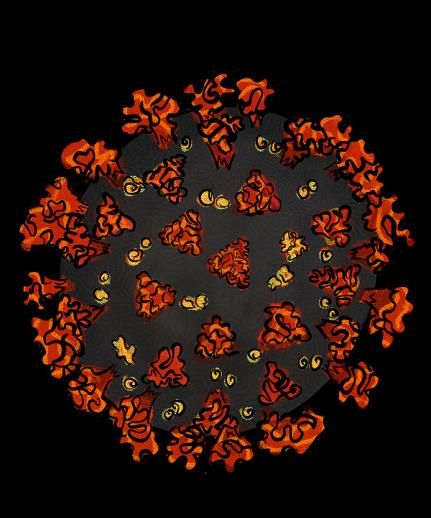
Figure 5 shows the box-plots of out-of-sample forecasting errors in the SDA horizon for
each model and dataset used. This horizon is chosen to analysis due to the recursive strategy
adopted, once the errors increase according to the growth of the forecasting horizon. The box
diagram depicts the variation of absolute errors for each model, which reflects the stability
of each model. In this context, the dots out of boxes are considered outliers errors, and the
black dot inside of the box is the MAE for each model.
AM BA CE MG PR
400
600
1500
750
300
200
400
1000
500
200
100
200
500
250
100
0
0
0
0
0
Absolute error
Stacking
Stacking
Stacking
Stacking
Stacking
CUBIST
CUBIST
CUBIST
CUBIST
CUBIST
ARIMA
ARIMA
ARIMA
ARIMA
ARIMA
RIDGE
RIDGE
RIDGE
RIDGE
RIDGE
SVR
SVR
SVR
SVR
SVR
RF
RF
RF
RF
RF
RJ RN RS SC SP
500
6000
200
400
1500
200
150
4000
300
1000
100
200
100
2000
500
50
100
0
0
0
0
0
Stacking
Stacking
Stacking
Stacking
Stacking
CUBIST
CUBIST
CUBIST
CUBIST
CUBIST
ARIMA
ARIMA
ARIMA
ARIMA
ARIMA
RIDGE
RIDGE
RIDGE
RIDGE
RIDGE
SVR
SVR
SVR
SVR
SVR
RF
RF
RF
RF
RF
Model
Figure 5: Box-plot for absolute error according to model and state for COVID-19 forecasting up to SDA
Through the box-plot analysis, boxes with lower size indicate models with lower variation
in the errors, and the results presented in Table A.1 are corroborated by the depicted in
11Figure 5. Models with lower errors also reach better stability, which means that the most
suitable modelling for each state can maintain a learning pattern, achieving homogeneous
prediction errors.
5. Conclusion and Future Research
In this paper, six machine learning approaches named CUBIST, RF, RIDGE, SVR,
and stacking ensemble, as well as ARIMA statistical model, were employed in the task of
forecasting one, three, and six-days-ahead the COVID-19 cumulative confirmed cases in ten
Brazilian states with a high daily incidence. The COVID-19 cumulative confirmed cases
for AM, BA, CE, MG, PR, RJ, RN, RS, SC, and SP states were used. The IP, MAE,
and sMAPE criteria were adopted to evaluate the performance of the compared approaches.
Moreover, the stability of out-of-sample errors was evaluated through box-plots.
In respect of obtained results, it is possible to infer that SVR and stacking-ensemble
learning model are suitable tools to forecast COVID-19 cases for most of the adopted states,
once that these approaches were able to learn the nonlinearities inherent to the evaluated
epidemiological time series. Also, ARIMA can be considered in some aspects for ODA, while
CUBIST and RIDGE models deserve attention for the development of this task in TDA
and SDA time windows. Therefore, the ranking of models in all scenarios is SVR, stacking
ensemble, ARIMA, CUBIST, RIDGE, and RF models. However, even though the models
discussed in this paper presented forecasting cases similar to those observed, they should be
used cautiously. This fact is attributed to the chaotic dynamics of the analyzed data, as well
as the diversity of exogenous factors that can affect the daily notifications of COVID-19.
For future works, it is intended (i) to adopt deep learning approaches combined to stacking
ensemble, (ii) to employ copulas functions for data augmentation dealing with small samples,
(iii) to use multi-objective optimization to tune hyperparameters of adopted models, (iv) to
adopt set of features which can help to explain the future cases of the COVID-19.
CRediT Author Statement
Matheus Henrique Dal Molin Ribeiro: Conceptualization, Methodology, Formal
analysis, Validation, Writing - Original Draft, Writing - Review & Editing. Ramon Gomes
da Silva: Conceptualization, Methodology, Formal analysis, Validation, Writing - Original
Draft, Writing - Review & Editing. Viviana Cocco Mariani: Conceptualization, Writing
- Review & Editing. Leandro dos Santos Coelho: Conceptualization, Writing - Review
& Editing.
Declaration of Competing Interest
The authors declare that they have no known competing financial interests or personal
relationships that could have appeared to influence the work reported in this paper.
12Acknowledgments
The authors would like to thank the National Council of Scientific and Technologic
Development of Brazil – CNPq (Grants number: 307958/2019-1-PQ, 307966/2019-4-PQ,
404659/2016-0-Univ, 405101/2016-3-Univ), PRONEX ‘Fundação Araucária’ 042/2018, and
Coordenação de Aperfeiçoamento de Pessoal de Nı́vel Superior - Brasil (CAPES) - Finance
Code 001 for financial support of this work.
References
[1] World Health Organization (WHO), . Coronavirus(COVID-19). 2020. URL: https:
//covid19.who.int/; (accessed in 22 April, 2020).
[2] Sohrabi, C., Alsafi, Z., O’Neill, N., Khan, M., Kerwan, A., Al-Jabir, A., et al. World
health organization declares global emergency: A review of the 2019 novel coronavirus
(COVID-19). International Journal of Surgery 2020;76:71–76. doi:10.1016/j.ijsu.
2020.02.034.
[3] Zhang, X., Ma, R., Wang, L.. Predicting turning point, duration and attack
rate of COVID-19 outbreaks in major western countries. Chaos, Solitons & Fractals
2020;:109829doi:10.1016/j.chaos.2020.109829.
[4] Boccaletti, S., Ditto, W., Mindlin, G., Atangana, A.. Modeling and forecasting
of epidemic spreading: The case of Covid-19 and beyond. Chaos, Solitons & Fractals
2020;doi:10.1016/j.chaos.2020.109794.
[5] Becerra, M., Jerez, A., Aballay, B., Garcés, H.O., Fuentes, A.. Forecasting emergency
admissions due to respiratory diseases in high variability scenarios using time series: A
case study in chile. Science of The Total Environment 2020;706:134978. doi:10.1016/
j.scitotenv.2019.134978.
[6] Fanelli, D., Piazza, F.. Analysis and forecast of COVID-19 spreading in china, italy
and france. Chaos, Solitons & Fractals 2020;134:109761. doi:10.1016/j.chaos.2020.
109761.
[7] Fong, S.J., Li, G., Dey, N., Crespo, R.G., Herrera-Viedma, E.. Composite monte carlo
decision making under high uncertainty of novel coronavirus epidemic using hybridized
deep learning and fuzzy rule induction. Applied Soft Computing 2020;doi:10.1016/j.
asoc.2020.106282.
[8] Roosa, K., Lee, Y., Luo, R., Kirpich, A., Rothenberg, R., Hyman, J., et al. Real-
time forecasts of the COVID-19 epidemic in China from february 5th to february 24th,
2020. Infectious Disease Modelling 2020;5:256 – 263. doi:10.1016/j.idm.2020.02.002.
13[9] Effenberger, M., Kronbichler, A., Shin, J.I., Mayer, G., Tilg, H., Perco, P.. Asso-
ciation of the COVID-19 pandemic with internet search volumes: A Google trendstm
analysis. International Journal of Infectious Diseases 2020;doi:10.1016/j.ijid.2020.
04.033.
[10] Davis, J.K., Gebrehiwot, T., Worku, M., Awoke, W., Mihretie, A., Nekorchuk,
D., et al. A genetic algorithm for identifying spatially-varying environmental drivers in
a malaria time series model. Environmental Modelling & Software 2019;119:275–284.
doi:10.1016/j.envsoft.2019.06.010.
[11] Ribeiro, M.H.D.M., da Silva, R.G., Fraccanabbia, N., Mariani, V.C., Coelho, L.d.S..
Forecasting epidemiological time series based on decomposition and optimization ap-
proaches. In: 14th Brazilian Computational Intelligence Meeting (CBIC). Belém, Brazil;
2019, p. 1–8.
[12] Scavuzzo, J.M., Trucco, F., Espinosa, M., Tauro, C.B., Abril, M., Scavuzzo, C.M.,
et al. Modeling dengue vector population using remotely sensed data and machine
learning. Acta Tropica 2018;185:167 – 175. doi:10.1016/j.actatropica.2018.05.003.
[13] Vaishya, R., Javaid, M., Khan, I.H., Haleem, A.. Artificial intelligence (ai) appli-
cations for covid-19 pandemic. Diabetes & Metabolic Syndrome: Clinical Research &
Reviews 2020;14(4):337–339. doi:10.1016/j.dsx.2020.04.012.
[14] Ribeiro, M.H.D.M., Coelho, L.d.S.. Ensemble approach based on bagging, boosting and
stacking for short-term prediction in agribusiness time series. Applied Soft Computing
2020;86(105837). doi:10.1016/j.asoc.2019.105837.
[15] Moreno, S.R., da Silva, R.G., Ribeiro, M.H.D.M., Fraccanabbia, N., Mariani, V.C.,
Coelho, L.d.S.. Very short-term wind energy forecasting based on stacking ensemble.
In: 14th Brazilian Computational Intelligence Meeting (CBIC). Belém, Brazil; 2019, p.
1–8.
[16] Justen, A.. Covid-19: Coronavirus newsletters and cases by municipality per day.
2020. URL: https://brasil.io/api/dataset/covid19/caso/data/?place_type=
state; (accessed in 20 April, 2020).
[17] Box, G.E., Jenkins, G.M., Reinsel, G.C., Ljung, G.M.. Time series analysis: fore-
casting and control. 5 ed.; John Wiley & Sons; 2015. ISBN 978-1-118-67502-1.
[18] Quinlan, J.R.. Combining instance-based and model-based learning. In: Proceedings of
the Tenth International Conference on International Conference on Machine Learning.
ICML’93; San Francisco, CA, USA: Morgan Kaufmann Publishers Inc. ISBN 1-55860-
307-7; 1993, p. 236–243.
[19] Rasmussen, C.E.. Gaussian Processes in Machine Learning; chap. 4. Heidelberg,
Germany: Springer. ISBN 978-3-540-28650-9; 2004, p. 63–71.
14[20] Hoerl, A.E., Kennard, R.W.. Ridge regression: Biased estimation for nonorthogonal
problems. Technometrics 1970;12(1):55–67. doi:10.1080/00401706.1970.10488634.
[21] Breiman, L.. Random forests. Machine Learning 2001;45(1):5–32. doi:10.1023/A:
1010933404324.
[22] Drucker, H., Burges, C.J.C., Kaufman, L., Smola, A.J., Vapnik, V.. Support vector
regression machines. In: Mozer, M.C., Jordan, M.I., Petsche, T., editors. Advances
in Neural Information Processing Systems 9. MIT Press; 1997, p. 155–161.
[23] Wolpert, D.H.. Stacked generalization. Neural Networks 1992;5(2):241–259. doi:10.
1016/S0893-6080(05)80023-1.
[24] Moreno, S.R., da Silva, R.G., Mariani, V.C., Coelho, L.d.S.. Multi-step wind
speed forecasting based on hybrid multi-stage decomposition model and long short-
term memory neural network. Energy Conversion and Management 2020;213(112869).
doi:10.1016/j.enconman.2020.112869.
[25] Kuhn, M.. Building predictive models in R using the Caret package. Journal of
Statistical Software, Articles 2008;28(5):1–26. doi:10.18637/jss.v028.i05.
[26] Hyndman, R., Athanasopoulos, G., Bergmeir, C., Caceres, G., Chhay, L., O’Hara-
Wild, M., et al. forecast: Forecasting functions for time series and linear models; 2020.
URL: http://pkg.robjhyndman.com/forecast; R package version 8.12.
[27] Hyndman, R.J., Khandakar, Y.. Automatic time series forecasting: the forecast
package for R. Journal of Statistical Software 2008;26(3):1–22. URL: http://www.
jstatsoft.org/article/view/v027i03.
[28] R Core Team, . R: A language and environment for statistical computing. R Foundation
for Statistical Computing; Vienna, Austria; 2018.
[29] Benvenuto, D., Giovanetti, M., Vassallo, L., Angeletti, S., Ciccozzi, M.. Application
of the arima model on the covid-2019 epidemic dataset. Data in Brief 2020;29(105340).
doi:10.1016/j.dib.2020.105340.
15Appendix A. Performance Measures
Table A.1 presents the performance measures for each model in each state and forecasting
horizon.
Table A.1: Performance measures for each evaluated model
Forecasting Model
State Criteria
Horizon ARIMA CUBIST RF RIDGE Stacking SVR
MAE 95 45 622.17 48.17 121.5 56.33
ODA
sMAPE 6.61% 2.80% 42.50% 2.83% 7.13% 3.18%
MAE 101.33 71.33 622.17 83.67 176.67 80.5
AM TDA
sMAPE 6.55% 4.50% 42.50% 4.49% 10.47% 4.19%
MAE 119.17 162.17 622.17 62.33 233.17 79.17
SDA
sMAPE 6.97% 9.55% 42.50% 3.45% 13.87% 4.13%
MAE 12 93.83 366.33 45.33 107.67 42.33
ODA
sMAPE 1.56% 9.16% 42.02% 4.36% 10.68% 4.15%
MAE 70 132 366.33 74.33 171.67 59.67
BA TDA
sMAPE 8.00% 12.92% 42.02% 7.46% 17.32% 5.63%
MAE 155.67 152.33 366.33 152.83 215.83 73.17
SDA
sMAPE 15.41% 15.08% 42.02% 15.16% 22.25% 6.90%
MAE 18 65.17 916 70.33 220.83 87.67
ODA
sMAPE 0.87% 2.49% 40.28% 2.81% 8.20% 3.17%
MAE 69.66 128.83 916 149.83 382.17 136.67
CE TDA
sMAPE 3.01% 4.48% 40.28% 5.39% 14.48% 4.78%
MAE 257 118.17 916 98.17 484.33 164.17
SDA
sMAPE 9.34% 4.11% 40.28% 3.52% 18.78% 5.77%
MAE 32 17.5 235.5 24.33 56.5 16
ODA
sMAPE 3.63% 1.81% 26.21% 2.50% 5.59% 1.57%
MAE 26 21.33 235.5 21.67 78.17 21
MG TDA
sMAPE 3.08% 2.20% 26.21% 2.13% 7.81% 2.04%
MAE 55 36.83 235.5 32.17 97.83 14.33
SDA
sMAPE 5.43% 3.58% 26.21% 3.14% 9.88% 1.41%
MAE 31 27.33 163.5 38 23.5 35.33
ODA
sMAPE 3.96% 3.26% 21.09% 4.50% 2.69% 4.18%
MAE 51.66 57.33 163.5 76.5 28.17 60.17
PR TDA
sMAPE 6.21% 6.56% 21.09% 8.61% 3.21% 6.89%
MAE 73.67 118 163.5 151 24.17 117.17
SDA
sMAPE 8.20% 12.56% 21.09% 15.75% 2.75% 12.53%
MAE 110 165.5 1305.67 273.67 69.5 360.83
ODA
sMAPE 3.17% 3.82% 37.06% 6.25% 1.70% 8.09%
MAE 120 275.67 1305.67 462.83 68 429.33
RJ TDA
sMAPE 3.18% 6.24% 37.06% 10.20% 1.65% 9.49%
MAE 158.33 532.67 1305.67 696.17 65.17 529.5
SDA
sMAPE 3.67% 11.34% 37.06% 14.67% 1.58% 11.43%
MAE 6 17 152.5 24.83 30.33 18.33
ODA
sMAPE 1.61% 3.87% 39.28% 5.56% 6.45% 4.14%
MAE 8.33 30.83 152.5 37.67 54 35.5
RN TDA
sMAPE 2.11% 6.54% 39.28% 8.51% 11.66% 7.69%
MAE 36.33 15.83 152.5 62 54 18.5
SDA
sMAPE 7.61% 3.42%% 39.28% 12.76% 11.66% 4.15%
MAE 12 12.83 146.67 11.33 45.5 8.17
ODA
sMAPE 1.64% 1.62% 19.82% 1.43% 5.76% 0.97%
MAE 24 19.17 147.33 18.67 71.33 8.5
RS TDA
sMAPE 3.22% 2.47% 19.92% 2.42% 9.14% 1.02%
MAE 34.5 34.17 147.5 37.67 91.83 7.83
SDA
sMAPE 4.31% 4.26% 19.95% 4.74% 11.89% 0.95%
MAE 21 93.67 179.5 180.5 33.83 177.67
ODA
sMAPE 2.43% 9.66% 20.97% 17.53% 3.66% 17.27%
MAE 44.33 100.33 179.5 277 41 257.33
SC TDA
sMAPE 4.76% 10.30% 20.97% 25.34% 4.39% 23.79%
MAE 56 102.83 179.5 338.5 43.83 330.33
SDA
sMAPE 5.65% 10.53% 20.97% 29.95% 4.68% 29.23%
MAE 436 1587 3799 537.33 1363.83 409
ODA
sMAPE 4.65% 13.47% 35.85% 4.44% 11.44% 3.51%
MAE 1485.66 2471.83 3801 579.17 2243 326.67
SP TDA
sMAPE 14.56% 21.81% 35.88% 4.79% 19.47% 2.77%
MAE 2779 3054.67 3801.5 591.83 2665.83 362.83
SDA
sMAPE 24.74% 27.60% 35.88% 4.95% 23.55% 3.04%
16Appendix B. Hyperparameters
Table B.1 presents the hyperparameters obtained by grid-search for the models employed
in this paper. In the stacking modeling, for the GP meta-learner there is no hyperaparameter
to be tuned.
Table B.1: Hyperparameters selected by grid-search for each evaluated model
Model
State ARIMA CUBIST SVR RIDGE RF
Number of randomly
(p,d,q) Committees Neighbors Cost Regularization
selected predictors
AM (1,2,0) 10 5 1 3.16E-03 2
BA (0,2,1) 20 9 1 1E-04 2
CE (2,2,1) 1 9 1 0 4
MG (0,2,1) 1 9 1 1E-04 2
PR (0,2,1) 20 5 1 3.16E-03 3
RJ (0,2,1) 1 9 1 1E-04 3
RN (1,1,0) 1 9 1 3.16E-03 5
RS (0,1,0) 1 9 1 1E-04 3
SC (0,2,1) 10 0 1 3.16E-03 5
SP (0,2,0) 20 9 1 1E-04 5
17You can also read