A mathematical model of lithosphere-atmosphere coupling for seismic events - Nature
←
→
Page content transcription
If your browser does not render page correctly, please read the page content below
www.nature.com/scientificreports
OPEN A mathematical model
of lithosphere–atmosphere
coupling for seismic events
Vincenzo Carbone1, Mirko Piersanti2*, Massimo Materassi3, Roberto Battiston4,5,
Fabio Lepreti1 & Pietro Ubertini2
Significant evidence of ionosphere disturbance in connection to intense seismic events have been
detected since two decades. It is generally believed that the energy transfer can be due to Acoustic
Gravity Waves (AGW) excited at ground level by the earthquakes. In spite of the statistical evidence
of the detected perturbations, the coupling between lithosphere and atmosphere has not been so far
properly explained by an accurate enough model. In this paper, for the first time, we show the result of
an analytical-quantitative model that describes how the pressure and density disturbance is generated
in the lower atmosphere by the ground motion associated to earthquakes. The direct comparison
between observed and modelled vertical profiles of the atmospheric temperature shows the capability
of the model to accurately reproduce, with an high statistical significance, the observed temperature
fluctuations induced by strong earthquakes.
In the last two decades the observation of ionospheric disturbances that precede and follow earthquakes is one of
the most debated topic in the literature. The first detection of changes in ionospheric parameters (e.g., F region
critical frequency—foF2) associated to the Alaskan earthquake was reported in1. In general, it is well known
that the ionosphere is influenced from above by the solar activity, leading to the so-called solar wind-magneto-
sphere-ionosphere coupling2–5. On the other hand, the ionospheric medium can be influenced from below by
atmospheric waves generated in the neutral a tmosphere6. Since the principal origin of energy in atmosphere is
connected to the its most dense (i.e. lowest) layers, it is expected that ionospheric plasma perturbations could
be caused by both dynamic tropospheric process, such as cyclones, motion of weather fronts, jet streams7,8, and
strong tectonic/technogenic sources of atmospheric oscillations, such as earthquakes, tsunami, volcano erup-
tions etc.9–11. The hypothesis of causal link between ionospheric perturbation observations associated to seismic
activity and neutral atmosphere oscillations, leading to Acoustic Gravity Waves (AGW), was first proposed b y12.
AGW indicates one of the dispersion branches in atmospheric waves characterized by a period of approximately
5 minutes to 10 hours, and wavelength of 10 m to 1000 kilometers. Because of the viscous dissipation of the
short wave components, its wavelength increases with altitude, reaching hundreds of meters in the ionospheric
D layer (located at an altitude between ∼ 60 and ∼ 90 km) and ∼ 10 km in the F2 layer (located at an altitude of
∼ 400 km). Such waves are the fastest atmospheric oscillations creating upfront of perturbations able to reach the
ionosphere13. It is worth highlighting that AGWs are able to provide “fast” dynamic coupling between the lower
atmosphere and ionosphere, especially those characterized by wavelengths of ∼ 100 − 200 km and phase and
group velocities of ∼ 100 − 200 m/s8. In addition, during the last two decades there were several publications on
experimental data on AGW induced by the earthquake activity (e.g.14, and reference therein).
From a theoretical point of view, waves in the atmosphere, as in any other elastic medium, are a relaxing pro-
cess that appears in response to any perturbation of equilibrium state of the medium. Atmospheric waves may be
described using all theoretical provisions of acoustics of fluids and gases. As a consequence, the oscillations in
the atmosphere are described by equations that strictly depends on the pressure, inertia forces, and atmospheric
vortexes (cyclones and anticyclones), as result of pressure and Coriolis forces, neglecting the inertia term15,16.
In this paper we describe a quantitative model that reproduces with high statistical accuracy how pressure
and/or density disturbances can be generated in the lower atmosphere by the ground motion associated to an
earthquake and how these disturbances can propagate up to the high atmosphere as AGW. As a case study we have
1
Physics Department, Universitá della Calabria, Ponte Pietro Bucci, Rende, Cosenza, Italy. 2INAF-Istituto di
Astrofisica e Planetologia Spaziali, Rome, Italy. 3Institute of Complex Systems, ISC-CNR, via Madonna del Piano
10, Sesto Fiorentino, 50019 Florence, Italy. 4Physics Department, Universitá di Trento, Via Sommarive, Povo,
Trento, Italy. 5INFN-TIFPA, Via Sommarive, Povo, Trento, Italy. *email: mirko.piersanti@inaf.it
Scientific Reports | (2021) 11:8682 | https://doi.org/10.1038/s41598-021-88125-7 1
Vol.:(0123456789)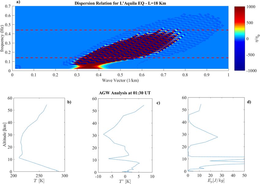
www.nature.com/scientificreports/
tested the model using data collected during four earthquakes, making a direct comparison between the observed
and modelled vertical profiles of the atmospheric temperature fluctuations induced by the different earthquakes.
Lithosphere: atmosphere coupling model
A seismic event manifests itself through surface waves detected by seismograms, whose dispersion relation is
described by Love-Reynolds17. The corresponding ground shaking induced by high-magnitude events can excite
perturbations at least in the first layer of the atmosphere, that we will call H.
Under the hypothesis that the wavelength involved in the perturbation are much grater than H, the dynam-
ics of the upper part of the layer can be roughly described within the shallow water approach18. For the sake
of simplicity we consider a 1D case, and define η(x, t) as the fluctuation amplitude of the top of the layer and
by u(x, t) the horizontal velocity. In the shallow water framework the time evolution of these quantities can be
described by two nonlinear equations that can be cast in a conservative form
∂η ∂
=− [(H + η − β)u] (1)
∂t ∂x
u2
∂u ∂
=− + gη (2)
∂t ∂x 2
where β is the “batimetry” of the ground (i.e. the impulsive perturbation of the ground), namely the finite shaking
of the ground due to the earthquake. The function β(x, t) could be extracted by usual seismograms. However,
for the sake of simplicity and without invoking a specific earthquake, we can assume that the impulsive event
can be described by a functional shape β(x, t) = β0 f (x, t)w(t), where f(x, t) represents the contribution of the
seismic surface waves, whose envelope is described by ω(t), related to the finite duration of the earthquake. Then
f (x, t) ∼ exp[i(ks x − ωs t)], where ωs /ks = vs is the phase speed of Love or Rayleigh surface waves, while, looking
at a typical seismograph, we can assume a specific functional shape for the envelope w(t) ∼ t exp(−αt 2 ), where
α −1/2 represents the Strong Motion Duration (SMD) of the seismic event, which is also related to the magnitude.
B y u s i n g t h e a n s a t z w h e r e b o t h φ(x, t) = [η(x, t); u(x, t)] a r e p r o p o r t i o n a l t o
φ(x, t) = k,ω φ(k, ω) exp[i(kx − ωt)] on the linearized equations (1), and by considering for simplicity that
the seismic event generates surface waves by a single component (ωs , ks ), after some algebra we get the surface
perturbation at the first atmospheric layer (see “Excited atmospheric modes during large earthquakes”), which
can be cast in a recursive form
η(k, ω) = F(k, ω)η(k − ks , ω − ωs ) (3)
where the function F is reported in “Excited atmospheric modes during large earthquakes”. The solution of (3)
allows us to obtain both the normalized amplitude of the perturbation and its dispersion relation (see “Excited
atmospheric modes during large earthquakes”). Using Eq. (15) in “Excited atmospheric modes during large
earthquakes”, we can obtain the wavemodes (k, ω) which can be excited by the earthquake.
Once the fluctuations have been generated roughly at the layer H ⋆ (H* being a characteristic altitude, see
"Excited atmospheric modes during large earthquakes"), they give rise to pressure fluctuation. In fact, a parcel
of atmosphere at H ⋆ , subject to the vertical displacement η from their equilibrium position, obtained from (15),
acquire a vertical velocity w in a way that the Lagrangian pressure fluctuation is given by19
p̃ = p − ρgw (4)
where p is the Eulerian pressure perturbation at a fixed point in space. By assuming the harmonic ansatz
exp[i(k · r − ωt)] for fluctuations, where k = (kx , ky ), the vertical dependence of both p̃ and w satisfy a set of
first-order ordinary differential e quations20
d p̃ gk2 g 2 k2
+ 2 p̃ =ρ ωd2 − 2 w (5)
dz ωd ωd
gk2
2
dw k 1 p̃
− 2w= − (6)
dz ωd ωd2 c02 ρ
where c0 is the sound speed, ρ is the mass density, and the intrinsic (Doppler-shifted) wave frequency ωd is defined
as ωd = ω − k · u , being u = (u, v) the horizontal velocity. These fluctuations can propagate as an acoustic-
gravity wave through the layered atmosphere, and the waveform at a given height z above H ⋆ can be investigated
by using the Wentzel-Kramers-Brillouin (WKB) a pproximation21 (see “Propagation of fluctuations through
atmosphere: a WKB approach”), thus obtaining the pressure fluctuations at a given height in the atmosphere.
As can be seen from Eq. (18) in “Excited atmospheric modes during large earthquakes”, the dispersion relation
of wave-vectors/frequencies, excited at height, H ⋆ strictly depends on specific earthquake parameters, namely:
the Peak Ground Acceleration (PGA), the length of the fault (L), the Strong Motion Duration (SMD - α), the
dominant seismogram frequency (ωs ) and the phase speed of the surface waves (vs).
Scientific Reports | (2021) 11:8682 | https://doi.org/10.1038/s41598-021-88125-7 2
Vol:.(1234567890)
www.nature.com/scientificreports/

                                             Date       Magnitude   L (km)   ωs (Hz)   PGA (g)   α (s)   vs (km/s)   ks · 10−5 (1/m)   H∗ (m)   ωt (Hz)
                                  Kobe       16/01/95   6.9         35       0.058     0.8       20      4.8         1.2               338      0.044
                                  Peru       23/06/01   8.2         35       0.036     0.3       40      1.6         2.2               203      0.051
                                  L’Aquila   06/04/09   5.9         18       0.05      0.5       33      1.5         3.3               395      0.43
                                  Fiji       19/08/18   8.2         50       0.01      0.77      35      4.5         0.2               161      0.072

                                  Table 1.  Parameters used for the evaluation of the pressure fluctuations dispersion relations associated to 1998
                                  Kobe, 2001 Peru, 2009 L’Aquila and 2018 Fiji earthquakes.

                                  Figure 1.  (a) Dispersion Relation evaluated for the Kobe Earthquake using the parameters in Table 1. The
                                  dashed line represents the parameter c0 /2h. (b) Vertical Temperature profile over the EQ epicenter. (c)
                                  Fluctuations of the vertical temperature profile over the EQ epicenter. (d) Potential energy density vertical
                                  profile over the EQ epicenter.

                                  Discussion
                                 We can investigate the dispersion relation wave-vectors/frequencies excited by a specific earthquake at height H ⋆ .
                                 As case studies we have investigated four earthquakes whose characteristic parameters are reported in Table 1.
                                 We obtained the earthquake parameters from the USGS dedicated website (www.usgs.gov/natural-hazards/
                                 earthquake-hazards/earthquakes). The dispersion relations of fluctuations for each earthquake, in the plane
                                 (k, ω), are reported in panel (a) of Figs. 1, 2, 3, 4 and 5. Experimental observations of AGW eventually detected
                                 over the earthquake epicenter are reported in panels (b), (c) and (d) of Figs. 1, 3, 4 and 5.
                                     Figure 1 shows the results obtained for 1995 Kobe earthquake. Looking at the dispersion relation it can be
                                 seen that fluctuations η(k, ω) have been roughly excited for wave-vectors ranging from 0.1 ≤ k ≤ 0.35 km−1,
                                 well above ks , and frequencies 0.1 ≤ ω ≤ 0.6 Hz well above ωs . Red dashed line in the panel a) represents the
                                 threshold (ωt = c0 /h, h being the temperature scale height) for the pressure fluctuations to propagate or do not
                                 propagate throughout the atmosphere up to the ionosphere, as purely vertical AGW, i.e. with k · u ≃ 0. In fact,
                                 as a consequence of Eq. (24), waves at frequencies ω excited by the seismic event, which satisfies ω2 > ωt2, are
                                 not evanescent and can propagate to high atmosphere. We evaluated ωt = 0.044Hz using the temperature profile
                                 retrieved from ERA5, which is the 5th generation atmospheric data set produced by the European Centre for

Scientific Reports |   (2021) 11:8682 |                 https://doi.org/10.1038/s41598-021-88125-7                                                             3

                                                                                                                                                          Vol.:(0123456789)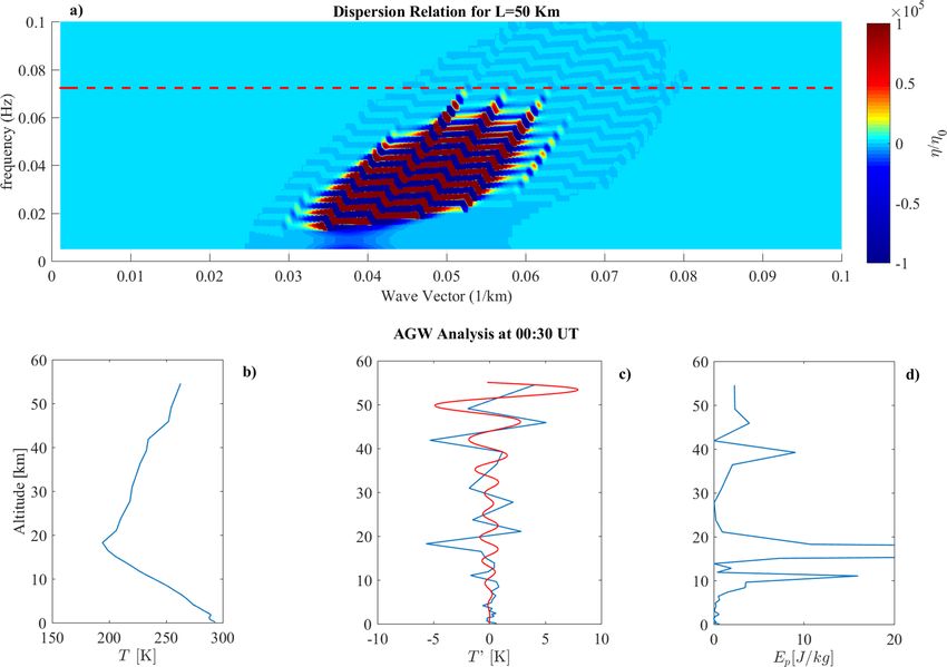
www.nature.com/scientificreports/
Figure 2. Box (A) Tri-dimensional dispersion relation evaluated for the Kobe Earthquake using the parameters
in Table 1. The dashed line represents the parameter c0 /2h. Box (B) Fluctuations of the vertical temperature
profile over the EQ epicenter (blue line) superimposed to the modelled temperature previsions at 21:00 UT.
Medium-Range Weather F orecasts22. As a result of our model, all the excited modes of η (panel a) can propagate
up to the ionosphere. So we expected to observe AGW injection in conjunction with the seismic event.
In order to check for possible AGW emission over the earthquake epicenter, we applied the method of
Piersanti et al. [ 2020]11. The results are presented in panels b), c) and d), displaying vertical atmospheric tem-
perature profile, the atmospheric temperature fluctuations with respect to a 3 km running average and the atmos-
pheric potential energy density, respectively, as obtained from ERA-5 database. A clear AGW propagation, char-
acterized by ∼ 2 km and ∼ 6 km wavelength, is detected in conjunction with the Kobe earthquake o ccurrence11.
Box (B) in Fig. 2 shows the direct comparison between the observed (blue line) and the modelled (red line)
temperature fluctuations vertical profile. The latter one can be estimated from the pressure fluctuations model
by using the equation of gas in atmosphere p̃(z) = ρ(z)R∗ T ′ (z), and a model profile for the atmospheric density
ρ(z) = ρ0 exp(−γ z), where R∗ = R/M , R is the gas constant, M = 28.97 g is the atmospheric mean molecular
mass, ρ0 = 1km/m3 and γ = 0.06 was atmospheric density mass decay i ndex23. The evaluation of the model tem-
perature was done by solving the Eq. (26) in “Propagation of fluctuations through atmosphere: a WKB approach”
for wave-vectors and frequencies obtained by the dispersion relation (Fig. 2 Box A). In particular we used the
three pairs corresponding to the maximum values of η/η0 (see Table 2) and T’(0)=0 as a boundary conditions.
The model is able to correctly reproduce the temperature fluctuation observations with a RMSE (root mean
square error) of 0.8 K and a correlation coefficient of 0.86. In addition, to determine whether there is a statistically
significant difference between the temperature fluctuations measured and the modelled one, we have performed a
χ 2 test (see Table 3 in “χ 2 test”), obtaining χ 2 = 47.3, suggesting that our model is able to reproduce the observa-
tions with > 90% probability. It is interesting to highlight that any phase shift due to a k · u transverse wave-vector
increases the χ 2 value. As a consequence, the pure vertical propagation represents the minimum χ 2 condition.
The same analysis has been repeated for the 23 June 2001 Peruvian earthquake. Looking at the dispersion
relation (Fig. 3a), we can see that fluctuations η(k, ω) have been roughly excited with wavevectors ranging from
0.1 ≤ k ≤ 0.72 km−1, well above ks, and frequencies 0.05 ≤ ω ≤ 0.8 Hz well above ωs. Also in this case our model
expected an AGW injection in conjunction with the earthquake occurrence, since all the excited modes of η are
greater than ωt = 0.051 Hz . This prevision is confirmed by the experimental vertical temperature profile and
potential energy density (panels b), c) and d). As for the Kobe event, we modelled the vertical behaviour of the
Scientific Reports | (2021) 11:8682 | https://doi.org/10.1038/s41598-021-88125-7 4
Vol:.(1234567890)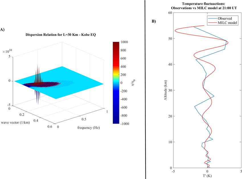
www.nature.com/scientificreports/
Figure 3. (a) Dispersion Relation evaluated for the Peru Earthquake using the parameters in Table 1. The
dashed line represents the parameter c0 /2h. (b) Vertical Temperature profile over the EQ epicenter. (c)
comparison between fluctuations of the vertical temperature profile observed (blue line) and modelled (red line)
over the EQ epicenter. (d) Potential energy density vertical profile over the EQ. epicenter.
temperature fluctuation using the three pairs corresponding to the maximum values of η/η0 (see Table 2). Even
in this case, the model is able to correctly reproduce the temperature fluctuation observations with a RMSE of
0.5 K and a correlation coefficient of 0.88. The χ 2 test confirms again that the model is able to reproduce the
observations with > 90% probability with a χ 2=48.8. Also in this case, we obtained that the pure vertical propaga-
tion represents the minimum χ 2 condition.
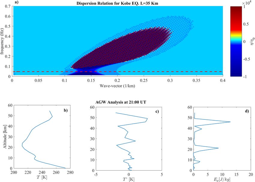
The third event analyzed is the 6 April 2009 L’Aquila earthquake, where ionospheric disturbances were not
observed. The analysis of experimental vertical temperature profile (Fig. 4b–d) confirms the lack of AGW injec-
tion over the earthquake epicenter. Figure 4a displays the dispersion relation, where η(k, ω) have been roughly
excited for wavevectors ranging from 0.28 ≤ k ≤ 0.8 km−1, well above ks , and frequencies 0.08 ≤ ω ≤ 0.44 Hz
well above ωs . However, in this case, all the excited modes are lower than ωt = 0.43Hz : in this case possibly
generated AGW are evanescent thus preventing a purely vertical propagation into the high atmosphere.
The analysis of the 19 august 2018 Fiji earthquake shows some peculiar features. In fact, the hypocenter of
the seismic event is situated at a large depth, about 300 km, and we observe that fluctuations at the first layer
in atmosphere (Fig. 5) have been excited for values of wave-vectors and frequencies lower than the previous
cases we analyzed. In particular, the modes excited have wave-vectors of the order of few tens of meters, and
frequencies of the order of a few tens of mHz, of the order of the surface waveform ks and ωs (Fig. 5a). The evalu-
ation of ωt ≃ 0.072 Hz, suggests that, in this case, the purely vertical propagation of AGW cannot be excited as
a consequence of the earthquake occurrence. However, experimental observations (Fig. 5b–d) show an AGW
propagation concurrently with the earthquake occurrence. In this case the discrepancy with our model predic-
tion is simply related to the absence of a purely vertical propagation. In fact, when we allow a phase shift due
to a weak transverse wave-vector, that is k · u ≃ 0.49 Hz, the excited fluctuation (corresponding to the pair: k1
=0.72 km−1 and ω1=0.43 Hz) can propagate as a quasi-vertical AGW, and the temperature profile is almost cor-
rectly reproduced by our model even in this particular case (Fig. 5c). In this conditions the RMSE is 2.8K and
the correlation coefficient ρ = 0.72. Finally, for the Fiji earthquake the χ 2 test gives worse result with reference
to previous events. In fact, we obtained χ 2=62.3, corresponding to 65% probability of the model to reproduce
the Fiji temperature fluctuations.
Conclusion
The possibility to correctly model, for the first time with high statistical significance, the lithosphere–atmosphere
coupling, i.e. how the pressure and density disturbance propagates in the upper atmosphere in case of large
earthquakes, is a breakthrough in the co- and post-earthquakes analysis. In particular, modelling how strong
Scientific Reports | (2021) 11:8682 | https://doi.org/10.1038/s41598-021-88125-7 5
Vol.:(0123456789)www.nature.com/scientificreports/
Figure 4. (a) Dispersion relation evaluated for the L’Aquila Earthquake using the parameters in Table 1.
The dashed line represents the parameter c0 /2h. (b) Vertical Temperature profile over the EQ epicenter. (c)
Fluctuations of the vertical temperature profile over the EQ epicenter. (d) Potential energy density vertical
profile over the EQ.
earthquakes can excite perturbations in the lower atmosphere that propagates vertically as AGW, allows a robust
statistical analysis that, in turn, provide a unprecedented tool to trim key parameters to fully reproduce the
observed perturbations. In addition, the model allows the a-priori simulation of earthquake effects in the high
atmosphere just during and after the event, and opens new scenarios to investigate, through a realistic physi-
cal model, co-seismic ionosphere disturbances due to high-magnitude earthquakes. This is a first step towards
forecasting earthquake effects in area known to be subjected to large release of energy triggered by tectonic,
volcanic etc, events.
More specifically, we have modelled the atmospheric fluctuations excited by a generic seismic event on the
top of the first layer of the atmosphere, and estimate its dispersion relation as a function of the characteristic
parameters of the earthquake. Then, using the Wentzel-Kramers-Brillouin (WKB) a pproach21, we model the pres-
sure fluctuations of the AGW excited by these near-ground fluctuations. The proposed model is able to provide
correct descriptions of AGW emission for three superficial earthquakes. For two of them, where the AGW are
expected to propagate and are actually observed11, the model provide a direct comparison between computed and
observed atmospheric vertical temperature profiles. It shows high reliability, with 90% of probability, to correctly
reproduce the temperature fluctuations induced by the earthquake with a low RMSE and correlation coefficient
larger than 0.86. The model is also able to correctly reproduce the case when ionosphere disturbances were not
observed, i.e. L’Aquila earthquake, showing that AGW should be evanescent.
The choice of an analytical model, despite the possible lower accuracy with respect to a numerical one, allows
to control and understand the physical process behind the atmosphere-lithosphere coupling system during
active seismic conditions. Finally, as shown in Fig. 6 for the KOBE case, the good statistical agreement between
the model and the data will allow to trim the model taking into account different earthquakes features, by the
use of a minimum χ 2 technique, while available a large data set, with small statistical error and low systematic
uncertainties.
Methods
Excited atmospheric modes during large earthquakes. Let us consider the linearized equations (1)
Scientific Reports | (2021) 11:8682 | https://doi.org/10.1038/s41598-021-88125-7 6
Vol:.(1234567890)www.nature.com/scientificreports/
Figure 5. (a) Dispersion Relation evaluated for the Fiji Earthquake using the parameters in Table 1. The dashed
line represents the parameter c0 /2h. (b) Vertical Temperature profile over the EQ epicenter. (c) Fluctuations of
the vertical temperature profile over the EQ epicenter. (d) Potential energy density vertical profile over the EQ.
Pair 1 Pair 2 Pair 3 RMSE (K) ρcorr
KOBE
k (km−1 ) 0.53 0.21 0.17 0.8 0.86
ω (Hz) 0.026 0.197 0.163
PERU
k (km−1 ) 0.8 0.48 0.11 0.5 0.88
ω (Hz) 0.51 0.43 0.15
Table 2. Parameters (k − ω ) used to model the temperature fluctuations over KOBE and PERU earthquake
epicenter.
∂η ∂u ∂β ∂u
+H =u +β (7)
∂t ∂x ∂x ∂x
∂u ∂η
+g =0 (8)
∂t ∂x
where, as well known, it is evident that the batimetry modifies the usual nondispersive oscillations described
by the classical relations dispersion ω2 /k2 = v02 = Hg . By assuming a flat soil, let us suppose now that a seismic
event modify impulsively the “batimetry” β(x, t), which represents here the shacking of the ground during the
earthquake. Introducing the Fourier series
φ(x, t) = φ(k, ω) exp[i(kx − ωt)]
(9)
k,ω
where φ means each of the variables η, u and β, from the linearized equations we get a pair of algebraic equations
Scientific Reports | (2021) 11:8682 | https://doi.org/10.1038/s41598-021-88125-7 7
Vol.:(0123456789)www.nature.com/scientificreports/
Altitude (km) ′
Tobserved (K ) ′
Tmodel (K ) ′
(Tobserved ′
− Tmodel )2 (K 2 )
54.59 −1.996 −1.919 0.005929
49.04 2.837 2.765 0.005184
45.84 2.557 1.0575 2.24850025
41.82 − 1.683 − 0.0454 2.68173376
39.17 − 0.671 1.072 3.038049
36.36 − 0.1293 0.5258 0.42915601
30.9 − 0.6216 − 0.5639 0.00332929
27.71 1.023 0.5922 0.18558864
23.69 − 1.879 0.3999 5.19338521
21.04 − 1.221 − 0.5355 0.46991025
18.23 − 0.1801 − 0.2988 0.01408969
16.48 0.2026 0.1239 0.00619369
15.04 − 0.09765 0.338 0.189790923
13.83 0.2817 0.5249 0.05914624
12.77 0.3952 0.4273 0.00103041
11.85 0.2606 0.2227 0.00143641
11.02 0.836 0.03857 0.635894605
9.582 − 0.7331 − 0.6579 0.00565504
8.368 − 0.8103 − 0.3217 0.23872996
7.317 − 0.382 − 0.368 0.000196
6.389 − 0.04751 − 0.009013 0.001482019
5.56 − 0.0165 − 0.09194 0.005691194
4.809 − 0.04025 − 0.08866 0.002343528
4.124 0.2105 0.05253 0.024954521
3.494 0.1537 0.4659 0.09746884
2.910 0.05543 0.02691 0.00081339
2.367 0.4936 − 0.2144 0.501264
2.109 0.05807 − 0.3863 0.197464697
1.859 0.09172 − 0.3475 0.192914208
1.616 − 0.1471 − 0.2124 0.00426409
1.381 − 0.01452 − 0.02012 0.00003136
1.153 0.03035 0.1232 0.008621123
0.9313 0.02111 0.3072 0.081847488
0.7156 0.05147 0.3021 0.062815397
0.5056 0.07786 0.2190 0.0199205
0.3011 0.07984 0.1021 0.000495508
0.1017 0.4315 0.1389 0.08561476
Table 3. Temperature fluctuations observed vs modelled for the Kobe earthquake.
ωu(k, ω) − kgη(k, ω) ei(kx−ωt) = 0
i
k,ω
−i [ωη(k, ω) − kHu(k, ω)]ei(kx−ωt)
k,ω
= u(p, w)ei(px−wt) iqβ(q, r)ei(qx−rt)
p,w q,r
+ ipu(p, w)ei(px−wt) β(q, r)ei(qx−rt)
p,w q,r
The Fourier coefficient of β(x, t) can be easily calculated
π 1/2 −ω2 /4α
β(k, ω) = β0 ei(kx−ωt) ωe δk,ks δω,ωs (10)
4α 3/2
so that the sum over the pair (q, r) can be eliminated by the delta functions, and, after anti-transforming, we
obtain the two following equations for the Fourier coefficients
Scientific Reports | (2021) 11:8682 | https://doi.org/10.1038/s41598-021-88125-7 8
Vol:.(1234567890)www.nature.com/scientificreports/
KOBE EQ temperature fluctuations
5
Observations
MILC
Temperature (K)
0
-5
-1 0 1 2
10 10 10 10
Altitude [km]
3
2
1
(data-model)/
0
-1
-2
-3
10-1 100 101 102
Altitude [km]
Figure 6. The figure shows, as an example, the comparison between observed (black circle) and modelled (red
line) fluctuations of the vertical temperature profile for KOBE EQ (Top panel); In the bottom panel are shown
the residuals with respect the model in 1σ units. As can be seen the model follows very well the data profile as a
function of the altitude with a good statistical approximation.
gk
u(k, ω) =
η(k, ω)
ω
β0 kωs 2
kHu(k, ω) − ωη(k, ω) =π 1/2 3/2 e−ωs /4α u(k − ks , ω − ωs )
4α
By inserting u(k, ω) into the second equation, we obtain a single equation for the perturbation coefficients
which can be cast in the recursive form
η(k, ω) − F(k, ω)η(k − ks , ω − ωs ) = 0 (11)
where the multiplicative factor is defined as
2
−1
π 1/2 β0 ωs e−ωs /4α ω ω2
F(k, ω) = 1− 2 2 (12)
4 v0 α 3/2 kv0 k v0
By interpreting k and ω in terms of the ground values κ = k/ks and ζ = ω/ωs , we can rewrite eq. (11) as
γ (ζ /κ)
η(κ, ζ ) − ψ(H, β, α, vs )
η(κ − 1, ζ − 1) = 0 (13)
1 − γ 2 (ζ /κ)2
where γ = vs /v0, the function ψ contains only parameters of the earthquake
Scientific Reports | (2021) 11:8682 | https://doi.org/10.1038/s41598-021-88125-7 9
Vol.:(0123456789)www.nature.com/scientificreports/
√
πg β ωs
−ω2 /4α
ψ(H, β, α, vs ) = √ e s (14)
4 H α
√
and β = β0 /g α is a dimensionless parameter.
The factorized form of Eq. (13) is particularly useful, because it can be solved recursively starting from
a reference value η0 = η(0, 0) which represents the unperturbed background at the surface eight H. Let us
consider a length scale L for wavevectors, and a time scale T for frequencies, then they can be enumerated by
using k = (2π/L)n and ω = (2π/T)m, where the pair (n, m) = 0, ±1, ±2, . . . are the integers of the wavevec-
tor-frequency plane. The shallow water approach requires L >> H , say kH H ⋆ , we can assume = rH ⋆ , where r is a free parameter, and L, the
length base, can be taken to be as an estimate of the seismic faulting. In this way
√ ⋆
αH r vs j
vi,j = (18)
ωs L v0 i
and the dispersion relation depends on the free parameters r and L. In our calculations of the dispersion relation
from real earthquakes, we used r = 10.
Propagation of fluctuations through atmosphere: a WKB approach. In the WKB framework,
assuming that the scale height of atmosphere h, the velocity u and the sound speed c0 are smooth function of
z/�, where represents some scale of variation of the variables, as a first-order approximation the Fourier coef-
ficient of pressure fluctuations at a given height z is related to that at H ⋆ through21
ωd2 ± img − g/2h
p(z) = p̃(z) (19)
ωd2 − g 2 k2 ωd−2
where
z
m(H ⋆ )A(z)
⋆
p̃(z) =p̃(H ) exp ±i m(z ′
)dz ′
+ ξ (20)
m(z)A(H ⋆ ) H⋆
Scientific Reports | (2021) 11:8682 | https://doi.org/10.1038/s41598-021-88125-7 10
Vol:.(1234567890)www.nature.com/scientificreports/
4
z dz ′ gk2 d ωd − g 2 k2
h 1 d
ξ= ln + ln (21)
H⋆ 2m ωd2 dz ′ ωd4 − g 2 k2 2h dz ′ ωd2
the vertical wavevector is defined as:
2
2
gk2 g 2 k2
1 ωd
m2 + − 2 = 1− 4 − k 2
(22)
2h ωd ωd c02
and the coefficient
g 2 k2
A = ρ ωd2 − 2 (23)
ωd
When the condition of propagation m2 > 0 is satisfied, either the upper and lower sign in (20) propagate as
oblique local plane waves. As m2 < 0 the wave is evanescent, while m2 (z̃) = 0 defines the so-called turning points
z̃ where WKB approximation fails. Moreover, WKB approximation diverges at points where either ωd = 0 or
ωd2 = kg . However, neither of these conditions exist for purely vertical propagation when k = 021. If we consider
quasi-vertically propagating waves, by assuming k c02 /4h2,
in order to be not evanescent and can propagate to high atmosphere. Under this condition, the pressure fluctua-
tions associated to quasi-vertically propagating waves, according to WKB, are
ω2 ± img − g/2h
p(z) ≃ p̃(z) (25)
ω2
where
z
m(H ⋆ )ρ(z)
⋆
p̃(z) ≃ p̃(H ) exp ±i m(z ′
)dz ′
(26)
m(z)ρ(H ⋆ ) H⋆
Equations (25) and (26) represents vertically propagating acoustic-gravity waves, with vertical wavevector
(24), generated from the perturbation of frequency ω excited at height H ⋆ by ground motion due to the large
earthquake.
χ 2 test. Here we show the table for the evaluation of the χ 2 test for the KOBE earthquake event and the com-
parison between the modelled and the observed atmospheric temperature fluctuations (Fig. 6).
Received: 31 December 2020; Accepted: 5 April 2021
References
1. Davies, K. & Baker, D. M. Ionospheric effects observed around the time of the alaskan earthquake of march 28, 1964. J. Geophys.
Res. (1896-1977) 70, 2251–2253, https://doi.org/10.1029/JZ070i009p02251 (1965). https://agupubs.onlinelibrary.wiley.com/doi/
pdf/10.1029/JZ070i009p02251.
2. Villante, U. & Piersanti, M. Sudden impulses at geosynchronous orbit and at ground. J. Atmos. Solar-Terrest. Phys. 73, 61–76.
https://doi.org/10.1016/j.jastp.2010.01.008 (2011).
3. Piersanti, M., Villante, U., Waters, C., Coco, I. The. & 8, ,. ulf wave activity: A case study. J. Geophys. Res. 117, https://doi.
org/10.1029/2011JA016857 (2012). Cited By 14 (2000).
4. Piersanti, M. et al. Comprehensive analysis of the geoeffective solar event of 21 June 2015: Effects on the magnetosphere, plasma-
sphere, and ionosphere systems. Solar Phys. 292, 169. https://doi.org/10.1007/s11207-017-1186-0 (2017).
5. Piersanti, M. et al. From the Sun to Earth: Effects of the 25 August 2018 geomagnetic storm. Ann. Geophys. 38, 703–724. https://
doi.org/10.5194/angeo-38-703-2020 (2020a).
6. Hines, C. O. Internal atmospheric gravity waves at ionospheric heights. Can. J. Phys. 38, 1441. https://doi.org/10.1139/p60-150
(1960).
7. Borchevkina, O., Karpov, I. & Karpov, M. Meteorological storm influence on the ionosphere parameters. Atmosphere 11, 1017
(2020).
8. Lizunov, G. & Hayakawa, M. Atmospheric gravity waves and their role in the lithosphere-troposphere-ionosphere interaction.
IEEJ Trans. Fundam. Mater. 124, 1109–1120. https://doi.org/10.1541/ieejfms.124.1109 (2004).
9. Pulinets, S. & Ouzounov, D. Lithosphere-atmosphere-ionosphere coupling (laic) model: An unified concept for earthquake pre-
cursors validation. Journal of Asian Earth Sciences 41, 371–382, https://doi.org/10.1016/j.jseaes.2010.03.005 (2011). Validation of
Earthquake Precursors-VESTO.
10. Yang, S.-S., Asano, T., Hayakawa, M. Abnormal. & gravity wave activity in the stratosphere prior to the, ,. kumamoto earthquakes.
J. Geophys. Res. 124, 1410–1425. https://doi.org/10.1029/2018JA026002 (2019). https://agupubs.onlinelibrary.wiley.com/doi/
pdf/10.1029/2018JA026002 (2016).
11. Piersanti, M. et al. bayan earthquake. Remote Sens. 12, 2020. https://doi.org/10.3390/rs12203299 (2018).
12. Hayakawa, M. & Fujinawa, Y. Electromagnetic Phenomena Related to Earthquake Prediction (Terra Scientific Publishing, 1994).
13. Galperin, Y. I. & Hayakawa, M. On the magnetospheric effects of experimental ground explosions observed from aureol-3. J.
Geomagn. Geoelectr. 48, 1241–1263. https://doi.org/10.5636/jgg.48.1241 (1996).
Scientific Reports | (2021) 11:8682 | https://doi.org/10.1038/s41598-021-88125-7 11
Vol.:(0123456789)www.nature.com/scientificreports/
14. Mikumo, T. & Watada, S. Acoustic-Gravity Waves from Earthquake Sources, 263–279 (Springer, Netherlands, Dordrecht, 2009).
15. W.H., H. Rossby-planetary waves, tides and gravity waves in the upper atmosphere, in Studies in Geophysics. The Upper Atmosphere
and Magnetosphere (The National Academies Press, Washington, DC, 1977).
16. Gossard, E., E, G., Hooke, W. & Hooke, W. Waves in the Atmosphere: Atmospheric Infrasound and Gravity Waves : Their Generation
and Propagation. Developments in atmospheric science (Elsevier Scientific Publishing Company, 1975).
17. Love, A. A Treatise on the Mathematical Theory of Elasticity (Cambridge University Press, Cambridge, 2013).
18. Vallis, G. K. Atmospheric and Oceanic Fluid Dynamics (Cambridge University Press, Cambridge, 2006).
19. Lamb, H., Lamb, H. & Caflisch, R. Hydrodynamics. Cambridge Mathematical Library (Cambridge University Press, 1993).
20. Pierce, A. D. Propagation of acoustic-gravity waves in a temperature-and wind-stratified atmosphere. J. Acoust. Soc. Am. 37,
218–227. https://doi.org/10.1121/1.1909317 (1965).
21. Godin, O. A. Wentzel–Kramers–Brillouin approximation for atmospheric waves. J. Fluid Mech. 777, 260–290. https://doi.org/10.
1017/jfm.2015.367 (2015).
22. Hennermann, K. & Berrisford, P. What are the changes from ERA-Interim to ERA5? available at https://confluence.ecmwf. int/
pages/viewpage.action?pageId=74764925 74764925 (2018).
23. Leslie, F. & Justus, C. The NASA Marshall Space Flight Center Earth Global Reference Atmospheric Model, 2010 Version. NASA
technical memorandum (National Aeronautics and Space Administration (Marshall Space Flight Center, Alabama, 2011).
Acknowledgements
The authors thank the two anonymous reviewers for their useful comments and suggestions. The parameters of
the earthquakes analysed in this manuscript are provided by USGS (https://earthquake.usgs.gov) datacatalogs.
ERA-5 data are processed and carried out by ECMWF within the Copernicus climate Change service (C3S), and
the data can be retreived from https://www.ecmwf.int/en/forecasts/datasets/reanalysis-datasets/era5. R. Battis-
ton and M. Piersanti thank the Italian Space Agency for the financial support under the contract ASI Limadou
Scienza + n° 2020-31-HH.0.
Author contributions
V.C. writing–original draft and formal mathematical analysis, M.P. writing–finalizing the manuscript, formal
analysis and methodology, M.M. formal mathematical analysis and validation, R.B. formal analysis, validation
and supervision, and P.U. writing–review and editing. All authors reviewed the manuscript and agreed to the
published version of the manuscript.
Competing interests
The authors declare no competing interests.
Additional information
Correspondence and requests for materials should be addressed to M.P.
Reprints and permissions information is available at www.nature.com/reprints.
Publisher’s note Springer Nature remains neutral with regard to jurisdictional claims in published maps and
institutional affiliations.
Open Access This article is licensed under a Creative Commons Attribution 4.0 International
License, which permits use, sharing, adaptation, distribution and reproduction in any medium or
format, as long as you give appropriate credit to the original author(s) and the source, provide a link to the
Creative Commons licence, and indicate if changes were made. The images or other third party material in this
article are included in the article’s Creative Commons licence, unless indicated otherwise in a credit line to the
material. If material is not included in the article’s Creative Commons licence and your intended use is not
permitted by statutory regulation or exceeds the permitted use, you will need to obtain permission directly from
the copyright holder. To view a copy of this licence, visit http://creativecommons.org/licenses/by/4.0/.
© The Author(s) 2021
Scientific Reports | (2021) 11:8682 | https://doi.org/10.1038/s41598-021-88125-7 12
Vol:.(1234567890)You can also read