Is Bitcoin a Relevant Predictor of Standard & Poor's 500? - MDPI
←
→
Page content transcription
If your browser does not render page correctly, please read the page content below
Journal of
            Risk and Financial
            Management

Article
Is Bitcoin a Relevant Predictor of Standard & Poor’s 500?
Camilla Muglia, Luca Santabarbara and Stefano Grassi *
    Department of Economics and Finance, University of Rome ’Tor Vergata’, Via Columbia 2, 00133 Rome, Italy;
    camilla.muglia@gmail.com (C.M.); luca-santa@hotmail.it (L.S.)
    * Correspondence: stefano.grassi@uniroma2.it

    Received: 14 May 2019; Accepted: 17 May 2019; Published: 31 May 2019

    Abstract: The paper investigates whether Bitcoin is a good predictor of the Standard & Poor’s 500
    Index. To answer this question we compare alternative models using a point and density forecast
    relying on Dynamic Model Averaging (DMA) and Dynamic Model Selection (DMS). According to
    our results, Bitcoin does not show any direct impact on the predictability of Standard & Poor’s 500
    for the considered sample.

    Keywords: cryptocurrency; Bitcoin; forecasting; point forecast; density forecast; dynamic model
    averaging; dynamic model selection; forgetting factors

1. Introduction
     The idea of cryptocurrency and the related technology, Blockchain, was suggested in 2009 by
an anonymous user known as Satoshi Nakamoto. He posted a paper to a cryptographic mailing list
introducing a new electronic cash system with very low transaction costs able to avoid the presence of
a central bank: the Bitcoin, see Nakamoto (2009). In the last ten years, cryptocurrencies have become
more and more popular among researchers and investors, with around 2000 cryptocurrencies available
at the time of writing. In recent months, the Bitcoin has experienced a dramatic price increase and
consequently, the global interest in cryptocurrencies has spiked substantially. Despite the price increase,
there are other numerous reasons for this intensified interest, just to mention a few: Japan and South
Korea have recognised Bitcoin as a legal method of payment (Bloomberg 2017a; Cointelegraph 2017);
some central banks are exploring the use of the cryptocurrencies (Bloomberg 2017b); a large number of
companies and banks created the Enterprise Ethereum Alliance1 to make use of the cryptocurrencies
and the related technology called blockchain (Forbes 2017). Finally, the Chicago Mercantile Exchange
(CME) started the Bitcoin futures on 18 December 2017, see Group (2017), Nasdaq and the Tokyo
Financial Exchange will follow, see Bloomberg (2017b).
     Although Bitcoin is a relatively new currency, there have already been some studies on this topic:
Hencic and Gourieroux (2015) applied a non-causal autoregressive model to detect the presence of
bubbles in the Bitcoin/USD exchange rate. The study of Cheah and Fry (2015) focused on the same
issue. Fernández-Villaverde and Sanches (2016) analysed the existence of price equilibria among privately
issued fiat currencies and Yermack (2015) wondered whether the cryptocurrency can be considered
a real currency. Sapuric and Kokkinaki (2014) measured the volatility of the Bitcoin exchange rate
against six major currencies. Chu et al. (2015) provided a statistical analysis of the log–returns of the
exchange rate of Bitcoin versus the USD. Catania and Grassi (2018) analysed the main characteristics of
cryptocurrency volatility.

1     Source: https://entethalliance.org/members/.

J. Risk Financial Manag. 2019, 12, 93; doi:10.3390/jrfm12020093                     www.mdpi.com/journal/jrfm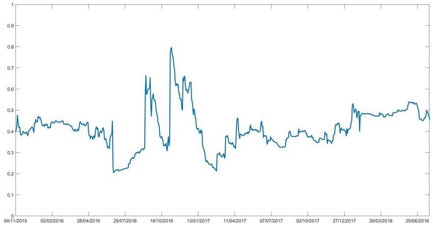
J. Risk Financial Manag. 2019, 12, 93                                                                            2 of 10

      Moreover Bianchi (2018) tried to investigate some of the key features of cryptocurrency returns
and volatilities, such as their relationship with traditional asset classes, as well as the main driving
factors behind the market activity. He found that returns on cryptocurrencies are moderately correlated
with commodities and a few more assets.
      Other studies have analyzed cryptocurrency manipulation and predictability. For instance,
Hotz-Behofsits et al. (2018) applied a time-varying parameter VAR with t-distributed measurement errors
and stochastic volatility. Griffin and Shams (2018) investigated whether Tether (another cryptocurrency
backed by USD) is directly manipulating the price of Bitcoin, increasing its predictability. Catania et al.
(2019) studied cryptocurrencies’ predictability using several alternative univariate and multivariate models.
They found statistically significant improvements in point forecasting when using combinations of
univariate models and in density forecasting when relying on a selection of multivariate models.
      Many institutions tried to investigate the relationship between Bitcoin and the stock market.
In some articles, it was speculated that the Bitcoin can improve stock market’s predictability, in this
case, Bitcoin could be used as a leading indicator. In an article by Bloomberg (2018), Morgan Stanley’s
analysts stated that “big investors may be dragging Bitcoin toward Market correlation”: the increasing
risk of this cryptocurrency may have had an attraction for investors who were seeking for high gains.
Stavroyiannis and Babalos (2019) examine the dynamic properties of Bitcoin and the Standard & Poor’s
500 (S&P500) index. They study whether Bitcoin can be classified as a possible hedge, diversifier,
or safe-haven with respect to the US markets. They found that it does not hold any of the hedge,
diversifier, or safe-haven properties and it exhibits intrinsic attributes not related to US markets.
      To the best of our knowledge, there are still no studies to confirm that Bitcoin is a good stock
market predictor. This paper tries to fill this gap, analyzing whether Bitcoin could be used as a leading
indicator for the S&P500.
      To answer this question, we allow for parameter and model uncertainty, avoiding Markov
Chain Monte Carlo (MCMC) estimation at the same time. This is accomplished using the
forgetting factors methodology (also known as discount factors) which have been recently proposed
by Raftery et al. (2010) and found to be useful in economic and financial applications, see Dangl
and Halling (2012) and Koop and Korobilis (2012) (KK). Another advantage of this methodology
is to provide, in close form, both the marginal and predictive likelihood (PL), which are useful in
model selection.
      The rest of the paper proceeds as follows: Section 2 presents the general model and the estimation
strategy; Section 3 presents the Dataset; Section 4 discusses the empirical results; finally, Section 5
reports some conclusions.

2. Models and Estimation Strategy
    Let yt ≡ (y1 , . . . , yt )0 denote the time series of interest and xt ≡ ( x1 , . . . , xt )0 the series of
exogenous variables, then the model can be written as:

                                        yt = zt γt + εt ,      εt ∼ N(0, Ht ),
                                                                                                                    (1)
                                        γ t = γ t −1 + η t ,   β t ∼ N(0, Qt ),

where yt is a scalar representing the observed time series at time t, zt = {yt−1 , . . . , yt− p , xt−1 , . . . , xt−q }
is a 1 × m vector (m = p + q) stacking all the lags of the series of interest and of the exogenous variable;
γt = {γ1,t , . . . , γ j,t } is an m × 1 vector containing the time varying states γs, which are assumed to
follow a random-walk dynamic. Finally, the errors, εt and β t , are assumed to be mutually independent
at all leads and lags. The Ht contains the time-varying volatilities of the series. The state space model
(SSM) of Equation (1) has been used in several recent papers, see among others, Primiceri (2005)
and Koop and Korobilis (2012).
      In order to estimate the quantities of interest, maximum likelihood or Bayesian estimation based
on MCMC can be used. However, these two estimation approaches end up being computationally
J. Risk Financial Manag. 2019, 12, 93 3 of 10
complex and, most of the time, infeasible. To reduce the computational burden, KK proposed two
main adjustments to the usual MCMC.
The first is to replace the variance-covariance matrix Qt with an approximation. Latent states—
γt —can then be obtained with a closed-form expression avoiding maximum likelihood or MCMC,
see Supplementary Materials. The second adjustment is to replace the measurement error variance
matrix Ht with an Exponential Weighted Moving Average (EWMA) type filter.
As discussed in Supplementary Materials, this methodology requires the specification of the
hyperparameters λ, α and κ and the specification of the initial condition of the states γ0 and Σ0 . Refer to
KK for an extensive discussion of the problem.
3. Dataset Description
Table 1 reports the dataset used for the analysis, with the transformation and the data source.
The sample goes from 11 August 2015 to 19 July 2018 and consists of 740 daily observations.
The crypto–market is open 24 h a day, seven days a week; hence, for computing returns we use
the closing price at midnight (UTC). As discussed in Catania et al. (2019), the data are available from
https://coinmarketcap.com/ with daily frequency; unfortunately, hourly data that could allow for a
more precise analysis are not freely available. To investigate non-stationary issues, three Unit-Root
tests have been performed: Augmented Dickey-Fuller (ADF) Test, Philips-Perron (PP) Test and
Kwiatkowsky, Phillips, Schmidt and Shin (KPSS) Test. All of them confirm the stationarity of each
transformed series, results are available from the authors upon request.
Table 1. Data overview and transformation. The table reports the series divided by type, Financial
predictors, Commodity predictors and Crypto predictors. The series are available for the period
11 August 2015 to 19 July 2018. For each variable the table reports the abbreviation code, the full name,
the data source and the transformation applied.
Code Full Name Transformation Data Source
Analyzed serie
S&P500 Standard & Poor’s 500 Log-First-Difference Thomson Reuters Eikon
Financial predictors
EF300 FTSEuroFirst300 Log-First-Difference Thomson Reuters Eikon
NASDAQ Nasdaq 100 Index Log-First-Difference Thomson Reuters Eikon
VIX CBOE Market Volatility Index Log-First-Difference Thomson Reuters Eikon
1mUS 1-month US Treasury Constant Maturity Rate First-Difference Federal Reserve System
10yUS 10-years US Treasury Constant Maturity Rate First-Difference Federal Reserve System
Commodity predictors
OIL ICE Brent Crude Eletronic Energy Future Log-First-Difference Thomson Reuters Eikon
GOLD SPDR Gold Shares Log-First-Difference Thomson Reuters Eikon
Crypto predictors
BTC Bitcoin Log-First-Difference Coinmarketcap
BHL Bitcoin High minus Bitcoin Low Log Coinmarketcap
Figure 1 reports Bitcoin closing price (BTC) which shows a steep rise in 2017 reaching the value
of almost 20,000 US dollars in December 2017. This ascending trend was severely interrupted at the
beginning of 2018, when price quickly dropped down to $6000. At the time of writing, BTC’s price is
fluctuating between 5000 and 6000 dollars.
The series reported in Table 1 are divided in: financial predictors, such as VIX; commodity
predictors, such as GOLD and crypto predictors such as BTC. Among the financial predictors, the VIX,
see Figure S1 in Supplementary Materials (Panel (c)), is the most volatile, as expected. It displays a
very steep peak between January and February 2018, the same period in which BTC’s price started
to fall.J. Risk Financial Manag. 2019, 12, 93 4 of 10
Table S1 in Supplementary Materials reports the correlation matrix of the predictors. As the
table shows the BTC appears to be highly positively correlated with all the financial indexes: S&P500,
EF300 and NASDAQ.
BTC Daily Closing Price
Figure 1. The figure reports the Bitcoin (BTC) closing price from August 2015 to July 2018. The plot
clearly shows the steep rise in the price 2017 and the sharp drop in 2018.
4. Analysis
The out-of-sample period begins on 1st September 2016 and the forecast horizon ranges from h = 1
to h = 7 days ahead. The analysis compares the performances of two models: the first—M1 —includes
all the predictors: financial, commodity and crypto predictors, see Table 1. The second, M2 , excludes
crypto predictors. The benchmark model, denoted with M0 , is an ARMA(1,1)-GARCH(1,1) model.
M1 and M2 can suffer from massive model uncertainty due to the number of possible predictor’s
combination at each time point t. For example, M1 has 29 = 512 models at each point in time.
To mitigate this fact, we use the DMA and DMS as described in Koop and Korobilis (2012) and
reported in Supplementary Materials. As already mentioned, the methodology requires fixing three
hyperparameters: the forgetting factor λ for the parameter variation; the decay factor κ for the EWMA;
and, finally, the discount weight α that weights each model based on forecast performances.
The results reported in this section are based on κ = 0.94. This value suits daily data,
see Riskmetrics (1996) and Prado and West (2010). The other parameters are set to α = 0.99 and
λ = 0.99, coherently with Raftery et al. (2010). In Section 4.2 a robustness analysis for the forgetting
factors α and λ is carried out. Moreover, we also tried to optimize at each time point λt using a standard
data-driven approach minimizing the expected prediction error. Unfortunately, the optimized λt with
crypto time series seems to be very unstable; we leave this issue as a topic of further research.
The analysis begins with the investigation of the posterior inclusion probabilities of each predictor:
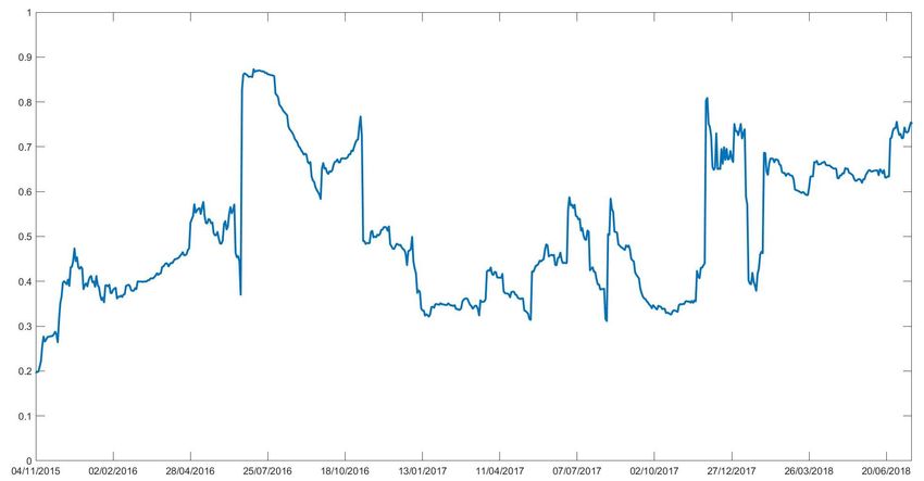
the higher the probability the higher the predictor’s influence over the dependent variable. Figure 2
depicts the posterior probabilities of BTC (Panel (a)), and of BHL (Panel (b)). Time-varying posterior
probabilities of inclusion for the other exogenous variables are reported in Supplementary Materials.J. Risk Financial Manag. 2019, 12, 93 5 of 10
(a) Posterior inclusion probability for BTC.
(b) Posterior inclusion probability for BHL.
Figure 2. Posterior inclusion probabilities. Panel (a) shows posterior inclusion probability for BTC.
Panel (b) shows posterior inclusion probability for BHL.
The figures show that the importance of each predictor switches rapidly over time, with a high
inclusion probability of BTC in some specific periods. One important change is in 2016 when the
inclusion probability suddenly jumped from 0.5 to 0.9 increasing the correlation with the S&P500 and
potentially its role as a leading indicator.
After a calm period during 2017, the BTC gained importance once again at the end of the same year
with a steep rise in price. During this period, a lot of articles pointed out a correlation between BTC and
financial markets. Bloomberg (2018) stated that “big investors may be dragging Bitcoin toward market
correlation” and see BTC as an asset which guarantees the highest potential risk/return combination in
the market. This may have attracted the interest of big investors able to move huge amounts of funds
and consequently correlate BTC to the USA stock market. Another article by Cointelegraph (2018)
asserted that BTC might be correlated with VIX, but there is no evidence that it may influence theJ. Risk Financial Manag. 2019, 12, 93 6 of 10
S&P500 index. An extensive analysis of the latter issue is carried out in the next sections using point
and density forecast.
4.1. Forecast Metrics
To assess the leading property of BTC we use point and density forecast. For the point forecasts,
we use the mean absolute forecast error (MAFE) for each forecast horizon, h = 1, . . . , 7:
T −h
1
MAFEh =
T−R ∑ ŷi,t+h|t − yi,t+h , (2)
t= R
where T is the number of observations, R is the length of the rolling window, ŷt+h|t is the S&P500
forecast made at time t for horizon h and yt+h is the realization.
To evaluate the density forecasts, we use predictive log score (LS) that is commonly viewed as the
broadest measure of density accuracy, see Geweke and Amisano (2010). As for the MAFE, we compute
the LS for each horizon:
T −h
s h ( yi ) = ∑ ln ( f (yt+h | It )), (3)
t= R
where f (yt+h | It ) is the predictive density for yt+h constructed using information up to time t.
We report the MAFEs and the LSs as a ratio of each model’s with respect to the baseline. Entries
smaller than 1 indicate that a given model yields forecasts that are more accurate than those from
the baseline and differences in score relative to the baseline, such as a negative number, indicates a
model that beats the baseline. In order to statistically assess the differences between alternative models,
we apply the Diebold and Mariano (1995) test for equality of the average loss (with loss defined as
squared error and negative log score) of each model versus the ARMA(1,1)-GARCH(1,1) benchmark
and we also employ the Model Confidence Set procedure of Hansen et al. (2011) using the R package
MCS detailed in Bernardi and Catania (2016) to jointly compare all predictions. Differences are tested
separately for each forecast horizon.
4.2. Point Forecast
Point forecast is evaluated through MAFE for both DMA and DMS as well as for their special
case, Bayesian Model Averaging (BMA). For each forecast horizon, the errors are calculated using
the following combination of forgetting and discount factors: λ = α = 0.99, λ = α = 0.95, λ = 1
and α = 0.99, λ = 0.99 and α = 1, and finally λ = α = 1. In all the cases, the decay factor is fixed to
κ = 0.94.
Table 2 compares point forecast for M1 and M2 as a ratio M0 (top) and against M0 (bottom).
From the upper table, it emerges that the errors are increasing in accordance with the forecast
horizon. Moreover, when h increases, the ratio increases, meaning that the benchmark model displays
better results than DMA and DMS. Table S8 in Supplementary Materials B shows that increasing the
forecasting horizon to h = 10 does not improve the forecasting performance of M1 and M2 . However,
Section 4.3, which analyses density forecasts results, reveals different outcomes.
Another peculiarity is that forecasts improve when α and λ tend to 1. When α = λ = 0.95 we
get the worst forecast performance for DMA and DMS, while the best results are obtained with BMA.
This may be due to the nature of the series: the presence of outliers and high peaks in BTC series may
distort the point forecast.
To see if BTC improves predictability over the S&P 500 a DM test is performed with a level of
significance equal to α = 95%. Results are reported in Supplementary Materials Table S2. There is no
evidence of an improvement in prediction when the BTC is added to the set of predictors. Further
results for different forecast horizons are reported in Supplementary Materials.
Using point forecast it seems that BTC does not improve predictability over the S&P 500 index.J. Risk Financial Manag. 2019, 12, 93 7 of 10
Table 2. Point forecast: M1 vs. M0 top table and M2 vs. M0 bottom table. Results are reported as the ratio between the model considered over the benchmark.
From both the tables it emerges that the simplest model, the ARMA(1,1)-GARCH(1,1), forecasts better than both DMA and DMS.
M1 vs. M0
DMA DMS DMA DMS DMA DMS DMA DMS BMA
λ = 0.99 λ = 0.99 λ = 0.95 λ = 0.95 λ = 0.99 λ = 0.99 λ=1 λ=1 λ=1
α = 0.99 α = 0.99 α = 0.95 α = 0.95 α=1 α=1 α = 0.99 α = 0.99 α=1
κ = 0.94
h=1 MAFE 1.006 1.000 1.063 1.089 1.013 1.011 1.014 1.013 1.026
h=2 MAFE 1.388 1.392 1.474 1.467 1.393 1.402 1.403 1.403 1.408
h=3 MAFE 1.651 1.668 1.760 1.798 1.651 1.659 1.667 1.655 1.658
h=4 MAFE 1.903 1.904 2.104 2.133 1.913 1.916 1.920 1.917 1.934
h=5 MAFE 2.121 2.125 2.368 2.401 2.118 2.118 2.151 2.150 2.188
h=6 MAFE 2.285 2.280 2.499 2.528 2.287 2.287 2.369 2.358 2.366
h=7 MAFE 2.481 2.466 2.699 2.702 2.483 2.482 2.619 2.621 2.611
M2 vs. M0
DMA DMS DMA DMS DMA DMS DMA DMS BMA
λ = 0.99 λ = 0.99 λ = 0.95 λ = 0.95 λ = 0.99 λ = 0.99 λ=1 λ=1 λ=1
α = 0.99 α = 0.99 α = 0.95 α = 0.95 α=1 α=1 α = 0.99 α = 0.99 α=1
κ = 0.94
h=1 MAFE 1.002 1.000 1.059 1.065 1.013 1.011 1.017 1.015 1.039
h=2 MAFE 1.386 1.387 1.462 1.460 1.391 1.390 1.403 1.402 1.403
h=3 MAFE 1.652 1.663 1.752 1.782 1.655 1.661 1.669 1.657 1.670
h=4 MAFE 1.904 1.910 2.112 2.128 1.908 1.910 1.917 1.914 1.923
h=5 MAFE 2.123 2.131 2.367 2.399 2.110 2.109 2.159 2.159 2.154
h=6 MAFE 2.288 2.289 2.506 2.527 2.291 2.295 2.385 2.374 2.386
h=7 MAFE 2.482 2.473 2.692 2.687 2.483 2.483 2.618 2.613 2.614J. Risk Financial Manag. 2019, 12, 93 8 of 10
4.3. Density Forecast
Density forecast is more informative than point forecast, as it is a measure of the prediction
uncertainty. The PL, which is the basis of density forecast, comes as a by-product of the adopted
estimation strategy. Table 3 reports the LS: the evidence is striking and the results are almost opposite
to those in Section 4.2. Both M1 and M2 provide statistically superior forecasts with respect to M0 .
Table 3. Log Score (LS), computed over the forecast horizon. Results are reported relative to the
benchmark specification (ARMA(1,1)-GARCH(1,1)) for which the absolute score is reported. Values in
bold indicate rejection of the null hypothesis of Equal Predictive Ability between each model and the
benchmark according to the Diebold-Mariano test at the 5% confidence level. Grey cells indicate those
models that belong to the Superior Set of Models delivered by the Model Confidence Set procedure at
confidence level 10%. As the table shows, the difference between M1 and M2 is very poor.
Days Ahead M0 M1 − M0 M2 − M0
h=1 −1659.997 −1023.949 −1024.600
h=2 −1651.352 −1767.424 −1763.904
h=3 −1647.144 −2188.181 −2187.612
h=4 −1643.063 −2496.529 −2498.355
h=5 −1639.526 −2733.322 −2740.850
h=6 −1636.366 −2930.505 −2927.831
h=7 −1631.968 −3097.841 −3093.876
The first column reports the PL for the benchmark model (M0 ), and the other columns report
the differences of M1 and M2 with respect to the benchmark. Among the three models, M0 shows the
worst results in contrast with the results of Section 4.2. The best forecast result is obtained for M1 when
h = 1; however, the difference between M1 and M2 is almost irrelevant. Following the same strategy
previously adopted the DM test is carried out, with a significance level of 95%.
The DM statistics, equal to −2.236, suggest that the null hypothesis of equal forecasting ability
is rejected. As discussed in Harvey et al. (1997), the DM test could be over-sized when the forecast
horizon is greater than one, so in those cases, we used the modified test given by:
i1/2
P+1−2h+ P−1 h(h−1)
h
S1∗ = P S1 ,
where S1 is the original statistics, h is the forecast horizon, P is the forecast evaluation period.
The modified version of DM test maintains the same null hypothesis of equal forecasting ability.
Whereas, the alternative is that model M2 is more accurate than model M1 .
H1 is accepted in this case since the test shows a very high p-value (0.987). In other words, model
M2 is performing better than M1 in terms of forecasting. Finally, the MCS indicates that DMS and
DMA has similar performance across horizons and they are both superior to the benchmark.
Therefore, the density forecast shows a different outcome to that of the point forecast. While the
benchmark model performs better than DMA and DMS in terms of MAFEs, the opposite is true when
the density forecast is considered. DMA and DMS give much better predictions for the S&P 500 when
the PL is considered.
The main goal of the paper is to understand whether BTC can be assumed to be a good predictor
for the S&P 500. Point forecast does not give any contribution to answering this question. A more
precise result is reached when the density forecast is used. Even though the PL are close to each other,
it has been found that the model that excludes the BTC related series outperforms the one that includes
them at lag one. For the other lags, the results are mixed and almost all the models are included
in the MCS without a clear superior model. This indicates that BTC does not seem to improve the
predictability of the S&P 500 index.
Table S9 in Supplementary Materials reports the results for α = λ = 0.99 and κ = 0.94 when
the Dow Jones (DJ) index is substituted to S&P500. It emerges that, using DJ, the BTC improves theJ. Risk Financial Manag. 2019, 12, 93 9 of 10
result of both point and density forecast for shorter horizon (one or two days ahead). These results are
promising and carrying out an extensive analysis for different markets is a topic for further research.
5. Conclusions
This work investigates whether BTC can be used as a leading indicator for the S&P500 index.
We use the methodologies recently introduced by Raftery et al. (2010), which allow the predictor’s weight
to change dynamically over time. The study is based on two distinct models: the first—M1 —includes
all the predictors; the second—M2 —excludes the crypto-predictors. The benchmark model—M0 —is
estimated using an ARMA(1,1)-GARCH(1,1).
The forecasting analysis is based on both point and density forecast. Results coming from the
point forecast are not very satisfactory: the M0 outperforms both M1 and M2 . Density forecast provides
a totally different outcome: M1 and M2 strongly outperform M0 . Unfortunately, in this case, the DM
and the MCS do not give clear evidence about which of the two models is the best. Accordingly,
from our results we can conclude that BTC does not show any predictive power over the S&P500 index.
In the coming years, cryptocurrencies will surely receive more and more consideration and there is the
possibility that our result may be disavowed.
Supplementary Materials: The supplementary materials are available online at http://www.mdpi.com/1911-
8074/12/2/93/s1.
Author Contributions: Conceptualization, C.M., L.S. and S.G.; methodology, S.G.; software, C.M., L.S. and S.G.;
validation, S.G.; formal analysis, C.M., L.S. and S.G.; investigation, C.M. and L.S.; data curation, C.M. and L.S.;
writing—original draft preparation, C.M. and L.S.; writing—review and editing, S.G.; supervision, S.G.; project
administration, S.G.
Funding: This research received no external funding.
Acknowledgments: We thank Francesco Ravazzolo for helpful comments.
Conflicts of Interest: The authors declare no conflict of interest.
References
Bernardi, Mauro, and Leopoldo Catania. 2016. Portfolio Optimisation under Flexible Dynamic Dependence
Modelling. Journal of Empirical Finance 48: 1–18. [CrossRef]
Bianchi, Daniele. 2018. Cryptocurrencies as an Asset Class? An Empirical Assessment. Technical Report, SSRN
Working Paper. Rochester: SSRN.
Bloomberg. 2017a. Japan’s BITPoint to Add Bitcoin Payments to Retail Outlets. Available online:
https://www.bloomberg.com/news/articles/2017-05-29/japan-s-bitpoint-to-add-bitcoin-payments-to-
100-000s-of-outlets (accessed on 29 May 2017).
Bloomberg. 2017b. Some Central Banks Are Exploring the Use of Cryptocurrencies. Available online:
https://www.bloomberg.com/news/articles/2017-06-28/rise-of-digital-coins-has-central-banks-
considering-e-versions (accessed on 28 June 2017).
Bloomberg. 2018. Big Investors May Be Dragging Bitcoin Toward Market Correlation. Available online:
https://www.bloomberg.com/news/articles/2018-02-07/big-investors-may-be-dragging-bitcoin-
toward-market-correlation (accessed on 7 February 2018).
Catania, Leopoldo, and Stefano Grassi. 2018. Modelling Crypto-Currencies Financial Time Series. Technical Report,
CEIS Working Paper. Glasgow: CEIS.
Catania, Leopoldo, Stefano Grassi, and Francesco Ravazzolo. 2019. Forecasting Cryptocurrencies under Model
and Parameter Instability. International Journal of Forecasting 35: 485–501. [CrossRef]
Cheah, Eng-Tuck, and John Fry. 2015. Speculative bubbles in Bitcoin markets? An empirical investigation into the
fundamental value of Bitcoin. Economics Letters 130: 32–37. [CrossRef]
Chu, Jeffrey, Saralee Nadarajah, and Stephen Chan. 2015. Statistical Analysis of the Exchange Rate of Bitcoin.
PLoS ONE 10: e0133678. [CrossRef] [PubMed]J. Risk Financial Manag. 2019, 12, 93 10 of 10
CME Group. 2017. CME Group Announces Launch of Bitcoin Futures. Available online: http://www.
cmegroup.com/media-room/press-releases/2017/10/31/cme_group_announceslaunchofbitcoinfutures.
html (accessed on 31 October 2017).
Cointelegraph. 2017. South Korea Officially Legalizes Bitcoin, Huge Market for Traders. Available online:
https://cointelegraph.com/news/south-korea-officially-legalizes-bitcoin-huge-market-for-
traders (accessed on 21 July 2017).
Cointelegraph. 2018. So Is There a Correlation Between Bitcoin and Stock Market? Yes, but No.
Available online: https://cointelegraph.com/news/so-is-there-a-correlation-between-bitcoin-and-stock-
market-yes-but-no (accessed on 13 February 2018).
Dangl, Thomas, and Mark Halling. 2012. Predictive Regressions with Time-Varying Coefficients. Journal of
Financial Econometrics 106: 157–81. [CrossRef]
Diebold, Francis, and Roberto Mariano. 1995. Comparing Predictive Accuracy. Journal of Business and Economic
Stastistics 13: 253–63.
Fernández-Villaverde, Jesus, and Daniel Sanches. 2016. Can Currency Competition Work? NBER Working Papers
22157. New York: National Bureau of Economic Research.
Forbes. 2017. Emerging Applications for Blockchain. Available online: https://www.forbes.com/sites/
forbestechcouncil/2017/07/18/emerging-applications-for-blockchain (accessed on 15 March 2012).
Geweke, John, and Gianni Amisano. 2010. Comparing and Evaluating Bayesian Predictive Distributions of Asset
Returns. International Journal of Forecasting 26: 216–30. [CrossRef]
Griffin, Jonh, and Amin Shams. 2018. Is Bitcoin Really Un-Tethered? Technical Report, SSRN Working Paper.
Rochester: SSRN.
Hansen, Peter, Asger Lunde, and James Nason. 2011. The Model Confidence Set. Econometrica 79: 453–97.
[CrossRef]
Harvey, David, Leybourne, Stephen, and Paul Newbold. 1997. Testing the equality of prediction mean squared
errors. International Journal of Forecasting 13: 281–91. [CrossRef]
Hencic, Andrew, and Christian Gourieroux. 2015. Noncausal Autoregressive Model in Application to Bitcoin/USD
Exchange Rate. In Econometrics of Risk. Studies in Computational Intelligence. Edited by Van-Nam Huynh,
Vladik Kreinovich, Songsak Sriboonchitta and Komsan Suriya. Cham: Springer, vol. 583.
Hotz-Behofsits, Christian, Florian Huber, and Thomas Zorner. 2018. Predicting Crypto-currencies Using Sparse
Non-Gaussian State Space Models. Journal of Statistical Software 37: 627–40. [CrossRef]
Koop, Gary, and Dimitris Korobilis. 2012. Forecasting Inflation Using Dynamic Model Averaging. International
Economic Review 53: 867–86. [CrossRef]
Nakamoto, Satoshi. 2009. Bitcoin: A Peer-to-Peer Electronic Cash System. Available online: https://Bitcoin.org/
Bitcoin.pdf (accessed on 31 October 2008).
Prado, Raquel, and Mike West. 2010. Time Series: Modeling, Computation, and Inference. Boca Raton: CRC Press.
Primiceri, Giorgio 2005. Time Varying Structural Vector Autoregressions and Monetary Policy. Review of Economic
Studies 72: 821–52. [CrossRef]
Raftery, Adrian. E., Miroslav Kárnỳ, and Pavel Ettler. 2010. Online Prediction under Model Uncertainty via
Dynamic Model Averaging: Application to a Cold Rolling Mill. Technometrics 52: 52–66. [CrossRef] [PubMed]
Riskmetrics. 1996. Riskmetrics—Technical Document, 4th ed. Technical Report. New York: J.P. Morgan/Reuters.
Sapuric, Svetlana, and Angelika Kokkinaki. 2014. Bitcoin is Volatile! Isn’t That Right? Paper presented at the
Business information Systems Workshops, Larnaca, Cyprus, May 22–23.
Stavroyiannis, Stavros, and Vassilios Babalos. 2019. Dynamic Properties of the Bitcoin and the US Market. Technical
Report. Rochester: SSRN.
Yermack, David 2015. Is Bitcoin a Real Currency? An Economic Appraisal. In Handbook of Digital Currency—Bitcoin,
Innovation, Financial Instruments, and Big Data. Cambridge: Academic Press, pp. 31–43.
c 2019 by the authors. Licensee MDPI, Basel, Switzerland. This article is an open access
article distributed under the terms and conditions of the Creative Commons Attribution
(CC BY) license (http://creativecommons.org/licenses/by/4.0/).You can also read