Wildfire Smoke Plume Segmentation Using Geostationary Satellite Imagery
←
→
Page content transcription
If your browser does not render page correctly, please read the page content below
Wildfire Smoke Plume Segmentation Using
                                    Geostationary Satellite Imagery

                                                  Jeff Wen 1 Marshall Burke 1 2

                          Abstract                                   tional Environmental Satellite (GOES) imagery (McNamara
                                                                     et al., 2004; Ruminski et al., 2007). We combine the meth-
       Wildfires have increased in frequency and sever-
                                                                     ods being developed in computer vision with geostationary
       ity over the past two decades, especially in the
                                                                     satellite imagery to identify wildfire smoke plumes in near
       Western United States. Beyond physical infras-
                                                                     real-time, providing a method to improve analysis with more
       tructure damage caused by these wildfire events,
                                                                     accurate identification of smoke and potentially extend anal-
       researchers have increasingly identified harmful
                                                                     ysis beyond the US.
       impacts of particulate matter generated by wildfire
       smoke on respiratory, cardiovascular, and cogni-              Researchers have applied machine learning techniques to
       tive health. This inference is difficult due to the           related problems with mixed results. Specifically, Wan et
       spatial and temporal uncertainty regarding how                al. (2011) used unsupervised learning approaches to clus-
       much particulate matter is specifically attributable          ter smoke in RGB color images using both a sharpening
       to wildfire smoke. One factor contributing to                 and mixture model approach (Wan et al., 2011). Their ex-
       this challenge is the reliance on manually drawn              ploratory results showed that it was possible to identify
       smoke plume annotations, which are often noisy                smoke plumes by analyzing satellite imagery, but the un-
       representations limited to the United States. This            supervised approach limited opportunities to examine the
       work uses deep convolutional neural networks to               out-of-sample performance of the models. Wolters and
       segment smoke plumes from geostationary satel-                Dean present two approaches to smoke segmentation by
       lite imagery. We compare the performance of                   combining labeled hyperspectral images with logistic re-
       predicted plume segmentations versus the noisy                gression models (Wolters & Dean, 2015; 2017). Their more
       annotations using causal inference methods to                 recent work illustrates the ability of auto-logistic regression
       estimate the amount of variation each explains                models to capture the spatial association between neigh-
       in Environmental Protection Agency (EPA) mea-                 boring pixels, which allows for smoothing over predictions.
       sured surface level particulate matter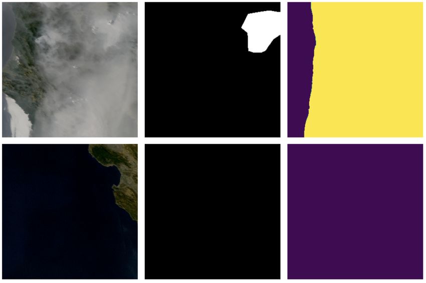
Wildfire Smoke Plume Segmentation

have allowed applied researchers to automate previously
manual, time-intensive annotation tasks with models that
can be trained and adapted to different problems.
Ramasubramanian et al. (2019) use a convolutional neural
network architecture with 6 bands of GOES-16 imagery as
input and HMS satellite-derived annotations that were sub-
sequently corrected by experts as labels (Ramasubramanian
et al., 2019). Their model uses a single timestamp as input
and relies on subject matter experts to manually correct the
imperfect labels, which resulted in a dataset size of approxi-
mately 120 scenes containing smoke. The authors note that
their model performs smoke pixel classification using the
pixel of interest in addition to an input neighborhood around
the pixel of interest. This approach results in predicted
boundaries that extend beyond the visible smoke boundary         Figure 1. First row: Model input, ground truth annotation label,
and relies on a manually defined input-pixel neighborhood        and model predicted segmentation after thresholding. Second row:
size. This along with the need for expert corrected labels       Additional input channel 07, channel 11, and MERRA-2.
makes it difficult to scale the approach to further analysis.
Larsen et al. (2021) utilize a fully convolutional network
(FCN) to identify wildfire smoke plumes from satellite ob-       models, we compare the predicted smoke plume segmenta-
servations obtained by the Himawari-8 geostationary satel-       tions against the HMS annotated smoke plumes on PM2.5
lite situated over East Asia and Western Pacific regions         measurements from EPA monitoring stations. Better under-
(Larsen et al., 2021). They use a deterministic cloud-           standing of the spatial extent of wildfire smoke is especially
masking algorithm to generate smoke versus non-smoke             important in downstream research, such as in the environ-
pixel labels, which are then used to train the FCN. While the    mental economics literature, where accurate identification
approach is similar, the manually annotated smoke plumes         of smoke plumes could lead to better estimates of the causal
in our work may better capture variability in the visual rep-    effect of smoke exposure.
resentation of smoke compared to a deterministic algorithm.
Other recent literature similarly use deep convolutional neu-    2. Methodology
ral networks (CNNs) for identifying smoke plumes from            2.1. Data
UAV and drone images as well as synthetically generated
smoke images (Frizzi et al., 2021; Yuan et al., 2019). These     The main imagery data used are satellite earth observations
works show promising performance but differ from the work        captured by the Geostationary Operational Environmen-
presented here as the aerial or synthetic images used provide    tal Satellite (GOES-16) positioned over the eastern United
a side-view angle of smoke rather than a top-down view. Li       States. GOES-16 along with the west coast GOES-17 satel-
et al. (2018) and Zhu et al. (2020) both use 3D convo-           lite provide frequent (every 5 minutes for the Continental
lution based CNN approaches to segment smoke plumes              US) multi-spectral measurements that are largely used for
from videos, but these video sequences also present a side-      weather modeling and storm tracking over the Atlantic and
viewing angle (Li et al., 2018; Zhu et al., 2020). While         Pacific oceans respectively. Images are downloaded if there
the side-view images may provide higher resolution, their        are associated smoke plumes during 2018 from the HMS
availability can be inconsistent compared to geostationary       annotations. In order to ensure that the imagery captures
satellite observations. Given the temporal frequency of geo-     radiance from the earth’s surface, images were limited to be-
stationary satellite imagery, future work can explore using      tween 12PM and 11PM Coordinated Universal Time (UTC).
video segmentation networks on sequences of geostationary        Furthermore, due to the large number of daily observations,
images.                                                          we limited training images to California and Nevada from
                                                                 the 2018 wildfire season between May-December of 2018.
In this work, we adapt CNNs to automatically identify wild-      However, we perform testing on unseen data between May-
fire smoke plumes from satellite imagery. We use satellite       October of 2019 and 2020. For testing on external data
observations as input and HMS annotated smoke plumes             from 2019-2020, we download 3 images per day between
as the target labels to train our models. Because analysts       May-October. These multiple images allow us to identify
often generate these plume annotations using multiple hours      if multiple plumes are overhead on a given day. Given the
of satellite imagery, we investigate different methods for       frequency of GOES imagery, in future work we hope to
improving training with these noisy labels. To validate our      increase the temporal resolution of the plumes.
Wildfire Smoke Plume Segmentation

                                                                In the rest of the paper, we will refer to the true-color image
                   Table 1. Input channels
                                                                as 1 band and the true-color, channel 07, and channel 11
  NAME           WAVELENGTH      T YPE       P RIMARY USES      combined as 3 bands. Lastly, 4 bands refers to using the
                                                                true-color, channel 07, channel 11, and the MERRA-2 in
  B LUE            0.47 µM     V ISIBLE     A EROSOLS
  R ED             0.64 µM     V ISIBLE C LOUDS & ASH           the input.
  V EGGIE          0.86 µM     N EAR -IR V EGETATION
  S HORTWAVE        3.9 µM        IR     F IRE HOTSPOTS         2.2. Model
  C LOUD -T OP      8.4 µM        IR       C LOUD - TOP
                                                                Our baseline experiments utilize an adapted U-Net neural
                                                                network architecture, originally designed for biomedical im-
After collecting the smoke plume data and the associated        age segmentation, to segment smoke plumes from a pseudo
GOES-16 imagery from the Amazon Web Services (AWS)              true-color RGB image (Ronneberger et al., 2015). The
NOAA open data repository, the raw imagery is reprojected       adapted network keeps the same number of layers in the
and a pseudo true-color composite is generated from the         encoding and upsampling blocks but decreases the number
red, blue, and ”green” bands using the SatPy package (Ras-      of convolutional filters. Furthermore, we replace the ReLU
paud et al., 2021). Although the GOES-16 satellite carries      activation function with PReLU activations for improved
multiple sensors, it lacks a green band, which must be gen-     stability in training. We also include multiple spectral bands
erated to create a true-color composite (Bah et al., 2018).     in subsequent experiments as these bands (shown in Table
Additionally, the 07 and 11 channels are also included in       1) provide contextual information of fire hotspot location
experiments as these near-infrared channels can be used for     and cloud-top phase in channel 07 and 11 respectively.
fire hotspot detection and cloud-top identification (examples   Across the model training, we use the Adam optimization
in Figure 1). Each of the downloaded images was saved           with a learning rate starting at α=5e-5 and stepping down by
as a 1200x1200 .geotiff image for a total of 615 im-            γ=0.1 every 9 epochs (Kingma & Ba, 2017). Each model
ages. These were then randomly cropped to generate up to        was trained for a total of 21 epochs using a batch size of 16.
15 different 300x300 images where 60% of the crops had a        We compared binary cross entropy (BCE) and mean abso-
smoke plume to deal with class imbalance. As a result, there    lute error (MAE) losses during the training and validation
were 6825 images which was split into 70% training, 15%         process. To track accuracy during training and validation,
validation, and 15% testing. We further ensured that the        we kept track of the average Dice coefficient.
cropped images generated from the same base image could
only be in one set of data to reduce potential data leakage.
                                                                                                    2|A ∩ B|
We pair the satellite imagery with smoke plume labels from                     Dice Coefficient =                          (1)
                                                                                                    |A| + |B|
the HMS archives. While the labels extend back to 2006,
we use observations from the most recent generation of
                                                                This statistical similarity metric first proposed by Lee Ray-
geostationary satellite (GOES-16) launched in mid-2017
                                                                mond Dice in 1945 and shown in Equation 1 calculates 2
as this subset of data allows for more spectral bands to be
                                                                times the amount of overlapping pixels between the pre-
used in the analysis. Analysts often use multi-hour ani-
                                                                dicted (A) and ground truth mask (B) divided by the total
mations to draw the extent of the smoke plumes, which
                                                                number of pixels in both masks (Dice, 1945).
presents challenges as the extent over time might not match
the boundaries of smoke plumes in a single image due to         Additionally, we consider two methods for explicitly han-
wind or other meteorological factors (Brey et al., 2018).       dling noisy labels in the training process. Specifically, we
Although the current labels are manually annotated from         experiment with using mean absolute value of error (MAE)
satellite imagery, one goal of this research is to identify     loss, which has been shown to be tolerant to label noise, and
the extent to which we can learn meaningful segmentations       data sampling to specify that only low loss training samples
from these imprecise labels. We attempt to improve train-       contribute to the gradient updates (Ghosh et al., 2017; Xue
ing on noisy labels by providing additional signal using the    et al., 2019). The loss sampling strategy allows the model to
Modern-Era Retrospective analysis for Research and Ap-          run the prediction on a batch of inputs as usual, but before
plications, Version 2 (MERRA-2) aersol optical thickness        calculating the average loss across samples, we identify the
(AOT) measurements of particulate matter as an additional       training sample in the batch that produced the highest loss.
input channel (Gelaro et al., 2017). The MERRA-2 data           Then, we set the loss for that example to 0 so that it does not
combines multiple sources of aerosol optical density in-        contribute to making weight updates. As mentioned by Xue
formation mainly derived from the Moderate Resolution           et al., this approach assumes that as the model performance
Imaging Spectroradiometer (MODIS) instrument aboard             improves, particularly noisy samples can result in high loss,
NASA’s Terra and Aqua satellites. We discuss 2 additional       which can have large impact on the weight updates. This
methods to account for the noisy labels in the next section.    training strategy mitigates the effect of these samples.
Wildfire Smoke Plume Segmentation
Table 2. Model performance on validation set. Bold rows represent
the models that achieve the best validation DICE coefficient for a
specific loss function. The asterisk denotes that the model weights
were updated after removing the highest loss sample per batch.
BANDS L OSS AVG . L OSS DICE
1 BCE 0.2535 0.0948
3 BCE 0.2236 0.1074
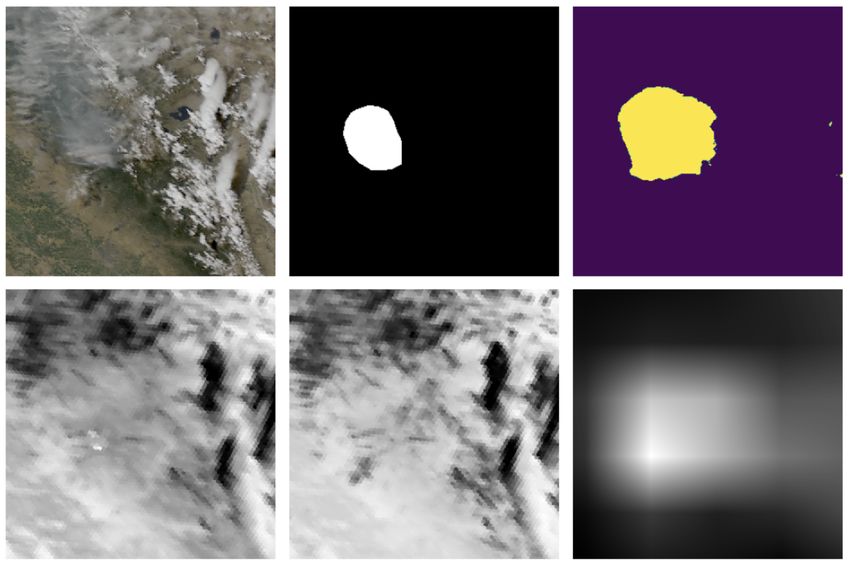
Figure 2. The model predicted segmentation on the right more 3* BCE 0.2313 0.1008
closely matches the visible smoke in the input imagery compared 4 BCE 0.1884 0.1028
to the HMS annotated smoke plumes in the middle, which cover 1 MAE 0.0986 0.2635
3 MAE 0.0986 0.2649
most of California. The input on the left is a test image from
3* MAE 0.0986 0.2655
September 8th, 2019 that was not used for training or validation. 4 MAE 0.0986 0.2655
2.3. External validation
While the DICE coefficient is used for validation during in PM2.5 measured at EPA monitoring stations explained
training, we apply the models on unseen images from 2019 by the smoke plumes and the W Adj.R2 metric represents
and 2020 to estimate the performance of these models com- the amount of variation in PM2.5 that is explained ”within”
pared to the hand annotated HMS smoke plumes from the the PM2.5 station unit by the different sources of smoke
same years. This allows us to test the models in a setting data. This distinction is important and we prefer the ”within”
most similar to downstream inference tasks where the mod- metric because it is a better indicator of ability to explain
els would be used to identify smoke plumes across a certain variation in PM2.5 using the different smoke data as it only
time frame, then used for additional analysis. considers remaining variation separate from time-invariant
unobserved station level differences.
Specifically, we leverage econometric tools for causally
identifying the contribution of wildfire smoke to changes
in ground level PM2.5 readings as measured by the EPA. 3. Results
We use a quasi-experimental approach to exploit variation Our preliminary results show that qualitatively the BCE loss
in smoke and PM2.5 over time to estimate the effect of models are able to learn to segment smoke from the input
identified wildfire smoke plumes on PM2.5 readings. We imagery. The top right panel in Figure 1 shows the perfor-
use fixed effect panel regressions (shown in Equation 2) with mance of the model on a validation sample and the rightmost
station fixed effects to account for time-invariant unobserved panel in Figure 2 and Figure 3 show segmentations of the
effects such as the fact that different stations may have model trained with BCE loss and 3 input channels on pre-
unobserved characteristics correlated with smoke exposure. viously unseen test images. The segmentations appear to
We set the station PM2.5 reading as the dependent variable more precisely locate the smoke in the input imagery on the
and consider the HMS annotations as well as different model left compared to the annotations in the middle. Even though
predicted smoke plumes as the independent variable. there is cloud cover in Figure 1, the model is able to learn to
differentiate between the cloud cover and the smoke plumes.
PM2.5it = β1 Smokeit + αi + it (2) Further quantitative results are shown in Table 2, where the
bolded rows represent the best validation DICE coefficient
when using either of the loss functions during training. The
This approach allows us to compare performance even in
asterisk denotes that the model weights were updated only
the presence of noisy annotation labels by measuring perfor-
after removing training samples that had the highest loss per
mance against an external ground truth. In the above equa-
batch (Xue et al., 2019).
tion, the αi captures the EPA station fixed effects, which
would handle time-invariant station level differences. The Although the MAE loss resulted in higher overall accuracy,
Smokeit variable is determined by the presence or absence the qualitative results indicated that these models were pre-
of smoke plumes overlapping an EPA station where the dicting ”no-smoke” for nearly all pixels and were unable to
smoke plumes come from either the HMS annotations or deal with the label imbalance in the images. Even with the
model predicted segmentations. addition of the additional step to sample only low loss train-
ing samples, the model performance with MAE loss was
To compare the HMS annotated smoke plumes against the
still qualitatively unable to identify smoke pixels compared
model predicted segmentations, we consider the adjusted R2
to the models trained with BCE loss.
(Adj.R2) and within-adjusted R2 (W Adj.R2) metrics.
The Adj.R2 metric measures the total amount of variation When we evaluate the model performance on previouslyWildfire Smoke Plume Segmentation
Table 3. HMS annotated vs. model predicted plume performance
on EPA PM2.5 measurements. Different sources of smoke plumes
are validated against external PM2.5 measurements using a fixed
effect panel regression approach to compare variation explained.
The asterisk denotes the loss sampling model results.
A DJ . R2 W A DJ . R2
A NNOTATIONS 0.2316 0.1946
1 BAND 0.2707 0.2367
3 BAND 0.2715 0.2374
4 BAND 0.3038 0.2703
3 BAND * 0.2987 0.2653
unseen data and compare the performance against the an-
notations, we see that the model predictions are able to ex- Figure 3. Additional examples show model predictions on unseen
test images with a lot of smoke in the first row and no smoke in
plain more of the variation in surface level PM2.5 readings
the second row. Model input, ground truth annotation label, and
regardless of model specification (results shown in Table
model predictions are displayed in both rows from left to right.
3). The higher values for the model predicted smoke data
suggest that while these results are preliminary, the CNN
segmented smoke plumes may explain more of the changes methods to compare the variation in EPA station PM2.5 mea-
in PM2.5 compared to the hand annotated smoke plumes. It surements that could be explained by either model predicted
is important to note that the hand annotations are meant to segmentations or hand annotated plumes. While smoke
capture visible smoke, while the particulate matter captured plumes have been manually annotated in the United States
at EPA stations might not be visible from satellite imagery. since the 2000s, our results suggest that automated segmen-
Therefore, the models leveraging the MERRA-2 channel as tation methods are at least qualitatively comparable to the
additional input might not be a fair comparison against the annotated smoke plumes and explain more of the within
hand annotations, which are mainly generated using visi- station PM2.5 variation in external validation. These early
ble imagery. However, as seen in Table 3, even the model results show the potential of adapting neural networks for
trained only using RGB as input appears to capture more of improving downstream inference even with noisy labels.
the ”within” station variation than the hand annotations. In future work, we look to focus on additional methods
While in Table 2 the model trained by removing the in- to improve the model robustness to noisy labels. We also
fluence of the highest loss sample per batch appeared to hope to extend and develop these methods to identify smoke
perform worse than the best 3-band model using BCE loss, across the globe and over time to better inform the impacts
in the external validation (shown in Table 3), this model of wildfires.
was able to explain more of the total and within variation in
PM2.5. Furthermore, this model was nearly able to match Software and Data
the performance of the 4-band model illustrating that ex- The Geostationary Operational Environmental Satel-
plicitly ignoring high loss training samples when there are lite (GOES) data used in this work is available
noisy labels could be beneficial for downstream tasks. This for download at https://registry.opendata.
might not be apparent from the validation accuracy metrics aws/noaa-goes. Hazard Mapping System smoke
because the validation dataset also includes noisy labels, data is available at https://www.ospo.noaa.gov/
which make it challenging to gauge model performance. Products/land. The models were developed using Py-
This underscores the importance of clean validation data Torch version 1.7.1 and the fixed effects estimators were
especially in the presence of noisy labels. estimated using the Fixest R package version 0.8.4 (Paszke
et al., 2019; Bergé, 2018). The models and data will be
4. Conclusion made available at the time of publication.
As wildfires continue to worsen, it is increasingly important
Acknowledgements
to quantify the effects of wildfire smoke exposure on soci-
ety. In this work, we used an adapted U-Net architecture to We thank reviewers whose comments and suggestions
segment smoke plumes from geostationary satellite imagery helped clarify and improve this manuscript. We also thank
with the goal of improving our understanding of the spatial the Sustainability and Artificial Intelligence Lab for discus-
extent of smoke. We further leveraged quasi-experimental sions.Wildfire Smoke Plume Segmentation
References //journals.ametsoc.org/view/journals/
clim/30/14/jcli-d-16-0758.1.xml.
Ba, R., Chen, C., Yuan, J., Song, W., and Lo, S. Smo-
kenet: Satellite smoke scene detection using convo- Ghosh, A., Kumar, H., and Sastry, P. S. Robust loss func-
lutional neural network with spatial and channel-wise tions under label noise for deep neural networks, 2017.
attention. Remote Sensing, 11:1702, 07 2019. doi:
10.3390/rs11141702. Hong, K. Y., Pinheiro, P. O., and Weichenthal, S. Predicting
global variations in outdoor pm2.5 concentrations using
Badrinarayanan, V., Kendall, A., and Cipolla, R. Segnet: satellite images and deep convolutional neural networks,
A deep convolutional encoder-decoder architecture for 2019.
image segmentation. CoRR, abs/1511.00561, 2015. URL
http://arxiv.org/abs/1511.00561. Kingma, D. P. and Ba, J. Adam: A method for stochastic
optimization, 2017.
Bah, M., Gunshor, M., and Schmit, T. Generation of goes-
16 true color imagery without a green band. Earth and Larsen, A., Hanigan, I., Reich, B. J., Qin, Y., Cope, M., Mor-
Space Science, 5(9):549–558, 2018. gan, G., and Rappold, A. G. A deep learning approach
to identify smoke plumes in satellite imagery in near-real
Bergé, L. Efficient estimation of maximum likelihood mod-
time for health risk communication. Journal of exposure
els with multiple fixed-effects: the R package FENmlm.
science & environmental epidemiology, 31(1):170–176,
CREA Discussion Papers, (13), 2018.
2021.
Brey, S. J., Ruminski, M., Atwood, S. A., and Fischer,
Li, T., Shen, H., Yuan, Q., Zhang, X., and Zhang,
E. V. Connecting smoke plumes to sources using haz-
L. Estimating ground-level pm2.5 by fusing satellite
ard mapping system (hms) smoke and fire location
and station observations: A geo-intelligent deep learn-
data over north america. Atmospheric Chemistry and
ing approach. Geophysical Research Letters, 44(23):
Physics, 18(3):1745–1761, 2018. doi: 10.5194/acp-
11,985–11,993, Dec 2017. ISSN 0094-8276. doi:
18-1745-2018. URL https://www.atmos-chem-
10.1002/2017gl075710. URL http://dx.doi.org/
phys.net/18/1745/2018/.
10.1002/2017GL075710.
Chung, Y.-S. and Le, H. Detection of forest-fire smoke
plumes by satellite imagery. Atmospheric Environment Li, X., Chen, Z., Wu, Q. J., and Liu, C. 3d parallel fully con-
(1967), 18(10):2143–2151, 1984. volutional networks for real-time video wildfire smoke
detection. IEEE Transactions on Circuits and Systems
Dice, L. R. Measures of the amount of ecologic association for Video Technology, 30(1):89–103, 2018.
between species. Ecology, 26(3):297–302, 1945.
Marmanis, D., Wegner, J. D., Galliani, S., Schindler, K.,
Filonenko, A., Kurnianggoro, L., and Jo, K.-H. Comparative Datcu, M., and Stilla, U. Semantic segmentation of aerial
study of modern convolutional neural networks for smoke images with an ensemble of cnss. ISPRS Annals of the
detection on image data. In 2017 10th International Photogrammetry, Remote Sensing and Spatial Informa-
Conference on Human System Interactions (HSI), pp. 64– tion Sciences, 2016, 3:473–480, 2016.
68. IEEE, 2017.
McNamara, D., Stephens, G., Ruminski, M., and Kasheta, T.
Frizzi, S., Bouchouicha, M., Ginoux, J.-M., Moreau, E., and The hazard mapping system (hms)–noaa multi-sensor fire
Sayadi, M. Convolutional neural network for smoke and and smoke detection program using environmental satel-
fire semantic segmentation. IET Image Processing, 15(3): lites. In 13th Conf. Satellite Meteorology and Oceanog-
634–647, 2021. raphy, 2004.
Gelaro, R., McCarty, W., Suarez, M. J., Todling, R., Mnih, V. Machine Learning for Aerial Image Labeling. PhD
Molod, A., Takacs, L., Randles, C. A., Darmenov, A., thesis, University of Toronto, 2013.
Bosilovich, M. G., Reichle, R., Wargan, K., Coy, L.,
Cullather, R., Draper, C., Akella, S., Buchard, V., Conaty, Paszke, A., Gross, S., Massa, F., Lerer, A., Bradbury,
A., da Silva, A. M., Gu, W., Kim, G.-K., Koster, R., J., Chanan, G., Killeen, T., Lin, Z., Gimelshein, N.,
Lucchesi, R., Merkova, D., Nielsen, J. E., Partyka, G., Antiga, L., Desmaison, A., Kopf, A., Yang, E., DeVito,
Pawson, S., Putman, W., Rienecker, M., Schubert, S. D., Z., Raison, M., Tejani, A., Chilamkurthy, S., Steiner,
Sienkiewicz, M., and Zhao, B. The modern-era retro- B., Fang, L., Bai, J., and Chintala, S. Pytorch: An
spective analysis for research and applications, version imperative style, high-performance deep learning
2 (merra-2). Journal of Climate, 30(14):5419 – 5454, library. In Wallach, H., Larochelle, H., Beygelzimer, A.,
2017. doi: 10.1175/JCLI-D-16-0758.1. URL https: d'Alché-Buc, F., Fox, E., and Garnett, R. (eds.), AdvancesWildfire Smoke Plume Segmentation
in Neural Information Processing Systems 32, pp. 8024– Xue, C., Dou, Q., Shi, X., Chen, H., and Heng, P. A. Robust
8035. Curran Associates, Inc., 2019. URL http:// learning at noisy labeled medical images: Applied to skin
papers.neurips.cc/paper/9015-pytorch- lesion classification, 2019.
an-imperative-style-high-performance-
deep-learning-library.pdf. Yuan, F., Zhang, L., Xia, X., Wan, B., Huang, Q., and Li,
X. Deep smoke segmentation. Neurocomputing, 357:
Ramasubramanian, M., Kaulfus, A., Maskey, M., Ra- 248–260, 2019.
machandran, R., Gurung, I., Freitag, B., and Christopher,
S. Pixel level smoke detection model with deep neural Zhu, G., Chen, Z., Liu, C., Rong, X., and He, W. 3d
network. In Image and Signal Processing for Remote video semantic segmentation for wildfire smoke. Machine
Sensing XXV, volume 11155, pp. 1115515. International Vision and Applications, 31(6):1–10, 2020.
Society for Optics and Photonics, 2019.
Raspaud, M., Hoese, D., Lahtinen, P., Finkensieper, S., Holl,
G., Dybbroe, A., Proud, S., Meraner, A., Zhang, X., Joro,
S., joleenf, Roberts, W., Ørum Rasmussen, L., Méndez, J.
H. B., Zhu, Y., Daruwala, R., strandgren, BENR0, Jasmin,
T., Barnie, T., Sigurosson, E., R.K.Garcia, Leppelt, T.,
ColinDuff, Egede, U., LTMeyer, Itkin, M., Goodson,
R., jkotro, and peters77. pytroll/satpy: Version 0.27.0
(2021/03/26), March 2021. URL https://doi.org/
10.5281/zenodo.4638572.
Ronneberger, O., Fischer, P., and Brox, T. U-net: Con-
volutional networks for biomedical image segmentation.
CoRR, abs/1505.04597, 2015. URL http://arxiv.
org/abs/1505.04597.
Ruminski, M., Kondragunta, S., Draxler, R., and Rolph,
G. Use of environmental satellite imagery for smoke
depiction and transport model initialization. In 16th An-
nual International Emission Inventory Conf.: Emission
Inventories—Integration, Analysis, and Communications,
2007.
Svejkovsky, J. Santa ana airflow observed from wildfire
smoke patterns in satellite imagery. Monthly Weather
Review, 113(5):902–906, 1985.
Wan, V., Braun, W. J., Dean, C., and Henderson, S. B. A
comparison of classification algorithms for the identifi-
cation of smoke plumes from satellite images. Statisti-
cal Methods in Medical Research, 20(2):131–156, 2011.
doi: 10.1177/0962280210372454. URL https://
doi.org/10.1177/0962280210372454. PMID:
20889573.
Wolters, M. A. and Dean, C. Issues in the identification of
smoke in hyperspectral satellite imagery — a machine
learning approach. 2015.
Wolters, M. A. and Dean, C. Classification of large-scale re-
mote sensing images for automatic identification of health
hazards. Statistics in Biosciences, 9(2):622–645, Dec
2017. ISSN 1867-1772. doi: 10.1007/s12561-016-9185-
5. URL https://doi.org/10.1007/s12561-
016-9185-5.You can also read