POWERPOINT PRESENTATION ON FINANCIAL MODELING SEMESTER -IV - INSTITUE OF AERONAUTICAL ENGINEERING COLLEGE - IARE

INSTITUE OF AERONAUTICAL ENGINEERING COLLEGE
                    (AUTONOMUS)

     POWERPOINT PRESENTATION
               ON
       FINANCIAL MODELING

                SEMESTER -IV

                 Ms. P.BINDU MADHAVI
                   ASSISTANT PROFESSOR
     DEPARTMENT OF MASTER OF BUSINESS ADMINISTRATION

UNIT-I

UNDERSTANDING THE BASIC
   FEATURES OF EXCEL

FINANCIAL MODELING

• Financial modeling is the construction of spreadsheet models
  that illustrate a company's likely financial results in
  quantitative terms. Financial models can simulate the effect of
  specific variables so that the company can plan a course of
  action should they occur.
• Financial modeling is the process by which a firm constructs a
  financial representation of some, or all, aspects of the firm or
  given security. The model is usually characterized by
  performing calculations and makes recommendations based on
  that information.
• The model may also summarize particular events for the end
  user such as investment management returns or the Sortino
  ratio, or it may help estimate market direction, such as the Fed
  model

DEFINITION

• “The process by which a firm constructs a financial
  representation of some, or all, aspects of the firm or
  given security. The model is usually characterized by
  performing calculations, and makes recommendations
  based on that information.
• The model may also summarize particular events for
  the end user and provide direction regarding possible
  actions or alternatives.”

TYPES OF FINANCIAL MODEL

• There are various kinds of financial models that are
  used according to the purpose and need of doing it.
  Different financial models solve different problems.
• While majority of the financial models concentrate
  on valuation, some are created to calculate and
  predict risk, performance of portfolio, or economic
  trends within an industry or a region.

DISCOUNTED CASH FLOW MODEL:

• Among different types of Financial model, DCF
  Model is the most important. It is based upon the
  theory that the value of a business is the sum of its
  expected future free cash flows discounted at an
  appropriate rate.

COMPARATIVE COMPANY ANALYSIS MODEL:

• Also referred to as the “Comparable” or “Comps”, it
  is the one of the major company valuation analyses
  that is used in the investment banking industry.
• In this method we undertake a peer group analysis
  under which we compare the financial metrics of a
  company against similar firms in industry. It is based
  on an assumption that similar companies would have
  similar valuations multiples, such as EV/EBITDA.

SUM-OF-THE-PARTS MODEL:

• It is also referred to as the break-up analysis. This
  modeling involves valuation of a company by
  determining the value of its divisions if they were
  broken down and spun off or they were acquired by
  another company.
•

LEVERAGED BUY OUT (LBO) MODEL:

• It involves acquiring another company using a
  significant amount of borrowed funds to meet the
  acquisition cost.
• This kind of model is being used majorly in leveraged
  finance at bulge-bracket investment banks and
  sponsors like the Private Equity firms who want to
  acquire companies with an objective of selling them
  in the future at a profit.

MERGER & ACQUISITION (M&A) MODEL:

• Merger & Acquisitions type of financial Model
  includes the accretion and dilution analysis. The
  entire objective of merger modeling is to show clients
  the impact of an acquisition to the acquirer’s EPS and
  how the new EPS compares with the status quo.
• In simple words we could say that in the scenario of
  the new EPS being higher, the transaction will be
  called “accretive” while the opposite would be called
  “dilutive.”

OPTION PRICING MODEL:

• On, to buy or sell the underlying instrument at a
  specified price on or before a specified future date”.
• Option traders tend to utilize different option price
  models to set a current theoretical value.

CUSTOMIZATION MICROSOFT EXCEL
               ENVIRONMENT:

• Personally I like the black colour, so my excel theme
  looks blackish. Your favourite colour could be blue, and
  you too can make your theme coulor look blue-like. If
  you are not a programmer, you may not want to include
  ribbon tabs i.e., developer. All this is made possible via
  customizations. In this sub-section, we are going to look
  at
• Customization the ribbon
• Setting the color theme
• Proofing settings
• Save settings

CREATING CHARTS

• Charts are used to display series of numeric data in a
  graphical format to make it easier to understand large
  quantities of data and the relationship between
  different series of data.

Dynamic formula method
•   Using our earlier sheet, you'll need five dynamic ranges: one for each series
    and one for the labels. Instructions for creating the dynamic range for the
    labels in column A follow. Then, use these instructions to create a dynamic
    label for columns B through E. To create the dynamic range for column A,
    do the following:
•   Click the Formulas tab.
•   Click the Define Names option in the Defined Names group.
•   Enter a name for the dynamic range, MonthLabels.
•   Choose the current sheet. In this case, that's DynamicChart1. You can use
    the worksheet, if you like. In general, it's best to limit ranges to the sheet,
    unless you intend to utilize them at the workbook level.
•   Enter the following formula:
•    =OFFSET(DynamicChart1!$A$2,0,0,COUNTA(DynamicChart1!$A:$A))
•   Click OK.

UNIT-II

SENSITIVITY ANALYSIS
    USING EXCEL

SENSITIVITY ANALYSIS USING EXCEL

The main goal of sensitivity analysis is to gain insight
into which assumptions are critical, i.e., which
assumptions affect choice.
The process involves various ways of changing input
values of the model to see the effect on the output
value. In some decision situations you can use a
single model to investigate several alternatives.
 In other cases, you may use a separate spreadsheet
model for each alternative.

ONE-VARIABLE DATA

• For a model with numerical input and numerical
  output, use the One Input One Output feature of the
  SensIt sensitivity analysis add-in.

LINE CHART OR XY (SCATTER) CHART:

The results of the Data table command may be displayed using
either a Line chart type or an XY (Scatter) chart type; both
types have a continuous numerical vertical axis.
However, the Line chart has a categorical horizontal axis,
which means that the worksheet data is displayed as equally
spaced text values. Only the XY (Scatter) chart has a
numerical horizontal axis.
Since the input values to a data table are usually equally-
spaced, you can use either chart type to display the results.
When the data for the horizontal axis are not equally-spaced, it
is important to use the XY (Scatter) chart type.

SCENARIO MANAGER

• The Scenario Manager is a great, but often
  overlooked What-If Analysis feature of Excel that
  will let you swap multiple sets of data in a worksheet
  and even compare them side-by-side. This technique
  can help you decide between multiple courses of
  action or what the implications are among several
  possibilities.
•

SENSITIVITY ANALYSIS

• A sensitivity analysis is a technique used to determine
  how different values of an independent variable
  impact a particular dependent variable under a given
  set of assumptions.
• This technique is used within specific boundaries that
  depend on one or more input variables, such as the
  effect that changes in interest rates have on bond
  prices.

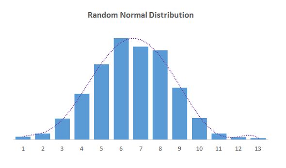
Random Normal Distribution

BUILDING MODELS IN FINANCE USING
                    SIMULATION

•   The projection model we will be developing is one that you might find as
    the starting point in many forms of analysis. The model will have these key
    features:
•   u It will have historical and forecast numbers for modeling an industrial
    type of company or business. Forecast numbers can be entered as ‘‘hard-
    coded’’ numbers (e.g., sales will be 1053 this year and 1106 next year,
    etc.) or as assumptions (e.g., sales growth next year will be 5 percent, etc.).
•   u The income statement, balance sheet, and a cash flow statement follow
    GAAP.
•   u The balance sheet balances: the total assets must equal the total liabilities
    and net worth. This balancing is done through the use of ‘‘plug’’ numbers
    (see Chapter 7). With the accounting interrelationships correctly in place,
    the cash flow numbers will also ‘‘foot’’ (see Chapter 11), i.e., the
    changes in cash flow must equal the change in the cash on the balance
    sheet.

UNIT-III

EXCEL IN ACCOUNTING

EXCEL IN ACCOUNTING:
• Microsoft Office Excel was designed to support
  accounting functions such as budgeting, preparing
  financial statements and creating balance sheets.
• It comes with basic spreadsheet functionality and many
  functions for performing complex mathematical
  calculations.
• It also supports many add-ons for activities such as
  modeling and financial forecasting, and seamlessly
  integrates with external data to allow you to import and
  export banking information and financial data to and from
  other accounting software platforms.

BALANCE SHEET ANALYSIS

• The common figure for a common-size balance sheet analysis is
  total assets. Based on the accounting equation, this also equals total
  liabilities and shareholders’ equity, making either term
  interchangeable in the analysis.
• It is also possible to use total liabilities to indicate where a
  company’s obligations lie and whether it is being conservative or
  risky in managing its debts.
• The common-size strategy from a balance sheet perspective lends
  insight into a firm’s capital structure and how it compares to rivals.
• An investor can also look to determine an optimal capital
  structure for an industry and compare it to the firm being analyzed.
  Then he or she can conclude whether debt is too high, excess cash is
  being retained on the balance sheet, or inventories are growing too
  high.

FORECASTING FINANCIAL STATEMENTS USING
                  EXCEL:

• Good forecasts must be consistent with historical
  performance and the current industry outlook.
• Look at historical numbers in relationship to others and
  use these ratios, particularly the operating ratios, to make
  your projections.
• All forecasts are estimates and approximations. Spend the
  time thinking and developing your ideas about the big
  picture, not the third decimal place.
• If the forecast looks too good to be true, it probably is.
• Re-examine your assumptions.

INCOME STATEMENT ACCOUNTS

• Revenues
• For industrial/manufacturing types of companies,
  revenues drive the other numbers in the model. Here are
  things to think about as you make your forecast:
• Revenues are the result of three main components: price,
  industry growth, and market share. Isolating the price
  growth from inflation will give you the measure for
  volume growth.
• Understand that in the context of the economic cycle, and
  then concentrate on what the drivers for future industry
  growth and market share might be.

ANALYZING FINANCIAL STATEMENTS BY USING
             SPREADSHEET MODEL:

•   Spreadsheets provide a roadmap of analysis. The maps present the big
    picture and delineate the “territories,” i.e., the major components of
    analysis. These maps help users keep the big picture in mind as they work
    through the details.
•   The spreadsheets provide a template that can be filled in with real data for
    hands-on illustrations.
•   The power of spreadsheets becomes apparent when one compares them to
    the traditional sequence of text narratives, algebraic derivations, numerical
    examples, and computations of metrics for real cases.
•   Spreadsheets condense this teaching material by an order of magnitude and
    enable what-if analyses.
•   In addition to condensing the material and presenting it using spreadsheets,
    our materials also clean up the terminology and provide a logical sequence
    of otherwise disparate topics. They show how valuation drives FSA.

DETERMINING PROJECT VIABILITY

•   Step 1: Research the Business Drivers
•   Step 2: Confirm the Alternative Solutions
•   Step 3: Determine the Feasibility
•   Step 4: Choose a Preferred Solution
•   Step 5: Reassess at a lower level

types of feasibility

• Economic feasibility, which uses economic analysis or
  cost/benefit analysis wherein the benefits are compared with
  the cost.
• Legal feasibility, which deals with the legal requirements.
• Operational feasibility, which deals with how to solve
  problems and take advantage of opportunities.
• Schedule feasibility, which deals with the duration of the
  development and completion of the system and if the schedule
  or deadline is desirable.
• Market and real estate feasibility, which involves testing of the
  geographical location of the project.
• Resource feasibility, which involves the amount of time set
  for the project and the type and amount of resources needed.

RISK ANALYSIS IN PROJECT APPRAISAL

• Analyzing the time to complete a project using project
  planning tools nearly always underestimates the time to
  completion. It is not the fault of the software or of the analysts,
  but of the use of 'best guess' values for task durations, etc. in
  the project plan. Risk analysis will allow you to avoid
  systematically underestimating project costs and durations.
• The project risk analysis course is designed to help those who
  wish to apply quantitative risk analysis modeling to project
  planning problems.
• A project is defined as any set of tasks involving resources
  (human, machine, time, financial) with well-defined goals.
  Project risk analysis aims at identifying the risks and
  uncertainties that threaten the achievement of those goals or
  the efficiency with which the project can be carried out.

RISK SIMULATION

• Risk simulation is a risk analysis technique that came
  to prominence in the early 1960s (Hertz, 1964 ). It
  involves the use of a probability distribution and
  random numbers, hence the Monte Carlo element, to
  estimate net cashflow figures. When discounted these
  figures sum to an estimated net present value (NPV)
  for a project. Repeated many times one gets a
  distribution of project NPV.

RESIDUAL INCOME MODEL (RIM)

• Along with the DDM, the residual income model (RIM)
  is another specialized version of a DCF used to value a
  firm. In its most basic form, the RIM has an equity charge
  that is equal to equity capital multiplied by the cost of
  equity.
• This is subtracted from net income to get to a residual
  income figure, which is used in lieu of cash flow or
  dividends, as calculated in the DCF and DDM models.
  Residual income figures can easily be modeled and
  calculated in Excel, but there are a number of steps to get
  to these calculations.

DETERMINATION OF VALUE DRIVERS:

• A value driver is an activity or capability that adds
  worth to a product, service or brand. More
  specifically, a value driver refers to those activities or
  capabilities that add profitability, reduce risk, and
  promote growth in accordance with strategic goals.
  Such goals can include increasing shareholder value,
  competitive edge and customer appeal.

DISCONTINUED CASH FLOW VALUATION:

•   The discounted cash flow (DCF) formula is equal to the sum of the cash
    flow in each period divided by one plus the discount rate Weighted Average
    Cost of Capital (WACC) raised to the power of the period number.

Here is the DCF formula:

•   DCF = (CF/(1+r)^1) + (CF/(1+r)^2) + (CF/(1+r)^3) + … + (CF/(1+r)^n)

Where:

•   CF = Cash Flow in the Period
•   i = the interest rate or discount rate
•   n = the period number

Steps in the DCF Analysis

• The following steps are required to arrive at a DCF
  valuation:
• Project unlevered FCFs (UFCFs)
• Choose a discount rate
• Calculate the TV
• Calculate the enterprise value (EV) by discounting the
  projected UFCFs and TV to net present value
• Calculate the equity value by subtracting net debt from
  EV
• Review the results

USING MODELS FOR RISK ANALYSIS

• Model inputs that are uncertain numbers -- we'll call
  these uncertain variables
• Intermediate calculations as required
• Model outputs that depend on the inputs -- we'll call
  these uncertain functions

UNIT-IV

EXCEL IN PORTFOLIO THEORY

DETERMINING EFFICIENT PORTFOLIO

• As we know, an efficient frontier represents the set of
  efficient portfolios that will give the highest return at
  each level of risk or the lowest risk for each level of
  return. A portfolio is efficient if there is no alternative
  with:
• Higher expected return with same level of risk
• Same expected return with lower level of risk
• Higher expected return for lower level of risk

FIXED INCOME PORTFOLIO MANAGEMENT USING
                 EXCEL:

• There are income funds which have a mandate to
  keep the maturity profile of the fund limited to some
  number. For E.g. Birla Dynamic normally keeps the
  duration near to 3. So how does one keep constant
  watch on it? How does one optimize return with
  respective duration? How should one allocate his
  funds to enjoy maximum convexity other things (i.e.
  duration, yield) remaining constant.

EXCEL IN DERIVATIVES BLACK
         SCHOLES IN EXCEL:

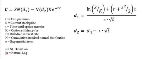
• The Black-Scholes formula (also called Black-
  Scholes-Merton) was the first widely used model for
  option pricing. It's used to calculate the theoretical
  value of European-style options using current stock
  prices, expected dividends, the option's strike price,
  expected interest rates, time to expiration and
  expected volatility.

• The formula, developed by three economists – Fischer
  Black, Myron Scholes and Robert Merton – is perhaps the
  world's most well-known options pricing model. It was
  introduced in their 1973 paper, "The Pricing of Options
  and Corporate Liabilities," published in the Journal of
  Political Economy. Black passed away two years before
  Scholes and Merton were awarded the 1997 Nobel Prize
  in Economics for their work in finding a new method to
  determine the value of derivatives (the Nobel Prize is not
  given posthumously; however, the Nobel committee
  acknowledged Black's role in the Black-Scholes model).

The Black-Scholes model makes certain assumptions:

• The option is European and can only be exercised at
  expiration.
• No dividends are paid out during the life of the option.
• Markets are efficient (i.e., market movements cannot be
  predicted).
• There are no transaction costs in buying the option.
• The risk-free rate and volatility of the underlying are
  known and constant.
• The returns on the underlying are normally distributed.

Black-Scholes Formula

REAL OPTIONS VALUATION

• The Real Options Valuation model encompasses a suite of
  option pricing tools to quantify the embedded strategic
  value for a range of financial analysis and investment
  scenarios.
• Traditional discounted cash flow investment analysis will
  only accept an investment if the returns on the project
  exceed the hurdle rate. While this is a worthwhile
  exercise, it fails to consider the myriad of strategic
  options that are associated with many investments.
• This model provides the ability to identify what options
  might exist in your proposal and the tools to estimate the
  quantification of them.

KEY FEATURES OF THIS MODEL

• Ease and flexibility of input, with embedded help prompts.
• Informative 'Quick Start' menu for choosing the correct tool
  for the situation.
• Modified Black Scholes options model to value the options to
  delay, expand, or abandon investments.
• Automatic binomial 'tree' builder model to evaluate complex
  strategic options with multiple stages.
• Nash equilibrium Game Theory model to evaluate market
  entry strategies in a competitive environment.
• Ability to predefine historical investment and/or industry risk
  profiles to utilize across real options models.
• Compatible with all versions of Excel for Windows as well as
  Excel for Mac as a cross platform analytical business solution.

UNIT-V

 UNDERSTANDING SUBROUTINES AND
   FUNCTIONS AND BUILDING SIMPLE
FINANCIAL MODELS USING SUBROUTINES
           AND FUNCTION

CHECK THE RECORDED CODE

• The Excel Macro Recorder created some code, while
  we performed the steps in our process. In my
  example, these were the steps:
• Open the orders file, named StationeryShort2007.xlsx
• Filter the list on the Data sheet, to show only the
  Binder orders
• Copy the Binder orders
• Create a new workbook
• Paste the Binder orders into the new workbook.

SUBROUTINES AND FUNCTIONS:

• Functions and subroutines are FORTRAN's subprograms.
  Most problems that require a computer program to solve
  them are too complex to sit down and work all the way
  through them in one go. Using subprograms allows you to
  tackle bite size pieces of a problem individually.
• Once each piece is working correctly you then put the
  pieces together to create the whole solution. To
  implement functions and subroutines, first write a main
  program that references all of the subprograms in the
  desired order and then start writing the subprograms.
• This is similar to composing an outline for an essay
  before writing the essay and will help keep you on track

TYPES OF FUNCTIONS AND SUBPROGRAMS

• Functions and subprograms can be grouped into
  several categories;
• Intrinsic or "built-in" functions
• Statement or "one-line" functions (Note: This link is
  optional)
• Function subprograms
• Subroutines

INTRINSIC FUNCTIONS

• The intrinsic functions are the set of "built-in" or
  library functions that all versions of FORTRAN
  provide. These are such things as SIN, COS, EXP,...
• The user of these functions "passes" one or more
  arguments to the function.
• e.g.,
   Y      =    COS(0.0)       ABMX      =   MAX   (A,B)
  0.0, A and B are called "arguments"

FUNCTION SUBPROGRAMS

• A FUNCTION subprogram is a "mini-program", that
  is, a collection of program statements which make it
  look like a program.
• Functions, being separate entities, perform separate,
  specific tasks.

PASSING ARGUMENTS

• Actual arguments are "passed" to the subprograms
  and used in place of the formal arguments. As
  previously stated, the actual arguments may have
  different names than the formal arguments BUT they
  must agree in NUMBER and TYPE.

DECISION RULES:

• A decision rule is a set of conditions that classify records.
  The rule predicts an outcome in the target field.

• Viewing the decision rules helps you determine which
  conditions are likely to result in a specific outcome. For
  example, consider some hypothetical decision rules that
  could predict churn.
• These rules might identify classifications based on the
  ranges for customer age and number of previous claims.
  From these rules, you might observe that customer who
  have no or 1 claim and are older than 50 are more likely
  to churn. The decision rule corresponds to a branch in a
  decision tree.

DEBUGGING

• To debug a program, user has to start with a problem, isolate the
  source code of the problem, and then fix it. A user of a program
  must know how to fix the problem as knowledge about problem
  analysis is expected. When the bug is fixed, then the software is
  ready to use. Debugging tools (called debuggers) are used to
  identify coding errors at various development stages.
• They are used to reproduce the conditions in which error has
  occurred, then examine the program state at that time and locate the
  cause.
• Programmers can trace the program execution step-by-step by
  evaluating the value of variables and stop the execution wherever
  required to get the value of variables or reset the program variables.
• Some programming language packages provide a debugger for
  checking the code for errors while it is being written at run time.

DEBUGGING PROCESS:

• 1.Reproduce the problem.
• 2. Describe the bug. Try to get as much input from
  the user to get the exact reason.
• 3. Capture the program snapshot when the bug
  appears. Try to get all the variable values and states
  of the program at that time.
• 4. Analyse the snapshot based on the state and
  action. Based on that try to find the cause of the bug.
• 5. Fix the existing bug, but also check that any new
  bug does not occur.

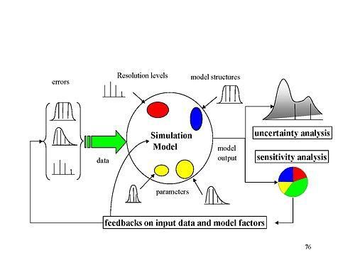
DESIGNING ADVANCED FINANCIAL MODELS USING
    VISUAL BASIC APPLICATION USER FORMS

• Automation is the buzz word in today’s corporate world.
  Whether it is manufacturing industry or the service
  industry, all businesses are aiming to reduce the human
  element for critical processes and tasks to improve
  efficiency and output.
• As a finance aspirant, you will see this trend in finance
  companies as well. Calculators are replaced by laptops,
  ledgers are replaced by spreadsheets and hard bound
  documented financial models are replaced by dashboards.
• If you want to pursue a career in finance, it is of utmost
  important for you to know the latest trends in your
  domain, and more importantly how to use automation in
  your day to day activities as a finance professional.

Advantages of Financial Modeling using VBA

•   1. Excellent output with minimum input
•   2. Speedy operations
•   3. Accuracy
•   4. Ease of comprehension

How to Create a Financial Model Using Excel and VBA?

•    1. Define the problem
•    2. Structure the logic
•    3. Identify the input variables
•    4. Define the output
•    5. Pilot run
•    6. Record/document the model
•    7. Monitor and update

ACTUAL MODEL BUILDING

• Step 1: Build Output Tabs Shell – Understand Your
  Requirements

• Step 2: Build Calculations on Paper – Determine
  Inputs Required

• Step 3: Build Input Tabs and Gather the Required
  Values

• Step 4: Load Data Tables
• Step 5: Build Calculations off of Inputs, Drivers, and
Data Tables
• Step 6: Link Calculated values to Output Tabs and
  Finalize Formatting of Output Tabs
• Step 7: Build Your Index Tab

• Step 8: Link Key Output Values to Drivers Tab to
  Perform Scenario and Sensitivity Analysis

• Step 9: Create Documentation and Finish Index Tab
• Step 10: Add Cell & Workbook Protection Where
  Appropriate

THE END