On possible types of magnetospheres of hot Jupiters
←
→
Page content transcription
If your browser does not render page correctly, please read the page content below

On possible types of magnetospheres of hot
                                                                    Jupiters
                                                                                   Zhilkin, A.G.∗, Bisikalo D.V.

                                                              Institute of Astronomy of Russian Academy of Sciences, Moscow, Russia
arXiv:1903.09459v1 [astro-ph.EP] 22 Mar 2019

                                               ABSTRACT. We show that the orbits of exoplanets of the “hot Jupiter” type, as a
                                               rule, are located close to the Alfv́en point of the stellar wind of the parent star. At
                                               this, many hot Jupiters can be located in the sub-Alfv́en zone in which the magnetic
                                               pressure of the stellar wind exceeds its dynamic pressure. Therefore, magnetic field of
                                               the wind must play an extremely important role for the flow of the stellar wind around
                                               the atmospheres of the hot Jupiters. This factor must be considered both in theoretical
                                               models and in the interpretation of observational data. The analysis shows that many
                                               typical hot Jupiters should have shock-less intrinsic magnetospheres, which, apparently,
                                               do not have counterparts in the Solar System. Such magnetospheres are characterized,
                                               primarily, by the absence of the bow shock, while the magnetic barrier (ionopause) is
                                               formed by the induced currents in the upper layers of the ionosphere. We confirmed this
                                               inference by the three-dimensional numerical simulation of the flow of the parent star
                                               stellar wind around the hot Jupiter HD 209458b in which we took into account both
                                               proper magnetic field of the planet and magnetic field of the wind.

                                               1         Introduction
                                                   When celestial bodies that have their own magnetic field interact with surrounding
                                               ionized matter, they create a cavity around themselves, which is named magnetosphere.
                                               In particular, such magnetospheres have Solar System planets blown over by the solar
                                               wind plasma [1]. The magnetosphere can have a complex structure and to change over
                                               the time, due to the heterogeneity and nonstationarity of the solar wind. Magnetic field of
                                               the planet prevents direct penetration of the solar wind plasma into the atmosphere. The
                                               boundary of the magnetosphere is a relatively thin current layer (magnetopause), which
                                               separates proper magnetic field of the planet from the magnetic field of the solar wind.
                                               Location of the magnetopause is determined by the balance of total pressure (the sum
                                               of the dynamic, gas, and magnetic pressure) from both sides of the boundary. However,
                                               in most cases, the total pressure from the outer side is equal to the dynamic pressure,
                                               while the pressure from the side of the planet is equal to the magnetic one. Such a
                                               situation exists, for instance, in the case of the Earth’s magnetosphere [2]. In the front
                                               of the magnetopause a bow shock forms, due to the supersonic flow regime. Between
                                                   ∗
                                                       E-mail: zhilkin@inasan.ru

                                                                                                1
shock and magnetopause, a transition region exists, in which the plasma of the wind is
heated, compressed, and retarded, changing the direction of the motion. An extended
magnetospheric tail forms at the night side.
    However, thousands of currently known exoplanets must have magnetospheres too.
Magnetospheres of the exoplanets may have their own specific features. In the present
paper, we will focus on the structure of the magnetospheres of the hot Jupiters. “Hot
Jupiters” are exoplanets with the mass comparable to the mass of Jupiter, located in
the immediate vicinity of the parent star [3]. The first hot Jupiter was discovered in
1995 [4]. Because of the proximity of the planets to the parent stars and their relatively
large size, gas envelopes of the hot Jupiters can overflow their Roche lobes, leading to the
formation of the outflows from the vicinities of the Lagrange points L1 and L2 [5,6]. This
is indirectly indicated by excessive absorption in the near-UV range, observed for some
planets [7–12]. These conclusions are confirmed theoretically by the one-dimensional
aeronomic models [3, 13–16].
    Based on the three-dimensional numerical modeling, it was shown in the series of
studies [17–23] that, depending on the parameters of a hot Jupiter, gas envelopes of three
main types can form [18]. To the first type belong closed envelopes, in which planet
atmosphere resides inside its Roche lobe. Into the second type fit open envelopes that are
formed by the outflows from the nearest Lagrange points. Finally, one can distinguish
quasi-closed envelopes of an intermediate type, for which stellar wind dynamic pressure
stops the outflow outside the Roche lobe. Calculations have shown that in the cases of
closed and quasi-closed envelopes the rate of mass loss by hot Jupiters is significantly
lower, compared to the case of open envelopes. Arakcheev et al. [24] presented results
of numerical modeling of the flow structure in the vicinity of the hot Jupiter WASP 12b
that took into account the influence of the planet’s magnetic field. It was shown that
the presence of even a relatively weak planet’s magnetic field (the magnetic moment
comprised 10 per cent of Jupiter’s magnetic moment) may lead to a noticeable decrease
of the rate of mass loss, compared to the net gas-dynamical case. In addition, magnetic
field may cause fluctuations in the outer parts of the envelope [25].
    There is an unaccounted factor in the studies quoted above, related to the magnetic
field of the stellar wind. However, the analysis performed in the present paper showed
that it is very important. The fact is that, apparently, many hot Jupiters are located in
the sub-Alfv́en zone of the stellar wind, where the magnetic pressure exceeds the dynamic
one. Therefore, accounting for magnetic field of the wind, formally, switches the flow of
the wind around a hot Jupiter from supersonic regime to subsonic one. As a result, in
this mode, bow shock should not form in the front of the atmosphere [26], i.e., the flow
is shock-less. This conclusion follows from the assumption that the magnetic field of
the wind is determined by the average magnetic field at the surface of the Sun, which
is about 1 G. However, magnetic fields of solar type stars can range from about 0.1
to several G [27, 28]. In addition, hot Jupiters can have parent stars not of solar type
only, because their spectral types are from F to M. The azimuthal component of the
magnetic field of the stellar wind is determined by the angular velocity of the stellar spin,
which, in turn, also depends on the spectral type [28]. If all these additional factors are
taken into account, it appears that some hot Jupiters may be located not only in the
transition region, separating the sub-Alfv́en and super-Alfv́en zones, but to move even
into the super-Alfv́en zone. This circumstance considerably expands the set of possible

                                             2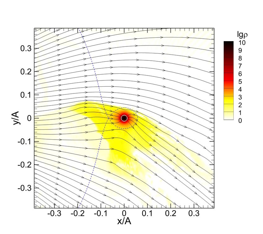
configurations of the magnetospheres of hot Jupiters.
   It should be noted that there is a simple way to approximate account of magnetic
wind field in the net gas-dynamical calculations. To do this, instead of gas pressure P ,
one needs to use full pressure PT = P + B 2 /(8π). It is not difficult to see that this is
equivalent to the replacement of the temperature T of the wind by the temperature

                                               u2A

                                   T̃ = T 1 + 2 ,                                     (1)
                                               2cT

where cT is the isothermal sound velocity, uA is the Alfv́en velocity. In this case, the
spatial distribution of the magnetic field B and, consequently, of the temperature T̃
should be determined by some kind of magnetohydrodynamical wind model. Such an
amendment can effectively increase the wind temperature and to switch the flow around
the planet into subsonic mode.
    In the present paper, we analyzed the possible types of magnetospheres of hot Jupiters,
taking into account possible outflows resulting from Roche lobe overflow. The results of
numerical simulations using three-dimensional magnetohydrodynamical model confirm
the conclusions obtained on the basis of simple theoretical considerations.
    The structure of the article is as follows. In §2 we describe the model of magnetic
field of the stellar wind applied by us. In §3 we analyze possible types of magnetospheres
of hot Jupiters. In §4 numerical model is described. In §5 results of calculations are
presented. The summary of the main results of the study follows in §6.

2    The model of magnetic field of the stellar wind
    In our numerical model, we will rely on the well-studied properties of the solar wind.
As it is shown by numerous ground- and space-based studies (see, for instance, the recent
review [29]), magnetic field of the solar wind has a rather complex structure. Schemati-
cally, this structure is shown in Fig. 1. In the corona region, magnetic field is essentially
non-radial, because there it is mainly defined by the own magnetic field of the Sun. At
the border of the corona, at the distance of several solar radii, the field, to a large ac-
curacy, becomes completely radial. Farther, heliospheric region is located, in which the
magnetic field to a substantial extent is determined by the properties of the solar wind.
In the heliosphere, with the distance from the center, magnetic field lines gradually twist
into a spiral due to the rotation of the Sun and therefore (especially at large distances)
the magnetic wind field can be described with a good accuracy using the simple Parker
model [30].
    However, the observed magnetic field in the solar wind is not axisymmetric and has
a pronounced sector structure. This is due to the fact that in the different points of
the spherical surface of the corona the field may have different polarity (direction of the
magnetic field lines relative to the direction of the normal vector), for example, due to
the inclination of the solar magnetic axis to the axis of its rotation. As a result, in
the ecliptic plane, in the solar wind form two clearly distinguished sectors with different
magnetic field directions. In one sector, magnetic field lines are directed to the Sun, while
in the opposite sector they are directed from the Sun. These two sectors are separated
by heliospheric current sheet, which is shown in Fig. 1 in gray. To the current sheet itself

                                             3
Fig. 1. Schematic picture of the solar wind in the ecliptic plane. Small dyed circle in the
center corresponds to the Sun. The arrow shows the direction of rotation of the Sun. The
boundary of the middle circle defines the corona region, at the border of which magnetic
field becomes completely radial. The shaded gray areas correspond to the zones of the
heliospheric current sheet which is shown by dashed lines running from the corona to
the periphery. It separates magnetic field of the solar wind with different directions of
magnetic field lines (from the Sun or to the Sun). The orbit of the planet (shown by
a dotted circle) is located in the heliospheric region. (A color version of the Figure is
available in the electronic version of the journal.

                                            4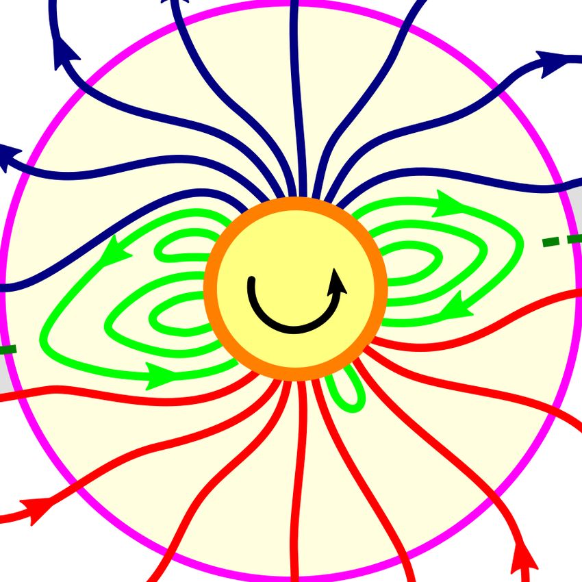
correspond two twisted dashed lines going from the border of the corona to the periphery
of the heliosphere. The heliospheric current sheet rotates with the Sun and, therefore, the
Earth, as it moves around the Sun, crosses it many times a year (about 13 times), moving
from the solar wind sector with one polarity of the magnetic field into the adjacent sector
with opposite polarity of the field.
    In this paper we do not take into account possible sectoral structure of the wind mag-
netic field, focusing on the impact of its global parameters. More detailed consideration
and account of the unquestionably important effects associated with the transition of the
planets through the current sheet and the polarity reversal of the magnetic field, we plan
to carry out in the further studies. On the top of everything else, in our model we will
assume that the orbit of a hot Jupiter is located in the heliospheric region beyond the
border of the corona. In Fig. 1 the orbit of the planet is shown as a large dotted circle.
    To the first approximation, to describe the magnetic field B of the wind in the he-
liospheric region, one can use the simple axisymmetric model described by Baranov and
Krasnobayev in the monograph [31]. In the inertial reference frame in the spherical co-
ordinates (r, θ, ϕ) magnetic field and stellar wind velocity can be represented as follows:

                  B = Br (r)nr + Bϕ (r, θ)nϕ ,   v = vr nr + vϕ (r, θ)nϕ .             (2)

At difference to [31], in these expressions we took into account the dependence of Bϕ
and vϕ on the angle θ, since our model is three-dimensional. More, for simplicity, in the
vicinity of the planet we will consider the radial component of velocity as constant and
equal to vw .
    In such an approximation, the structure of stellar wind is described by a system of
equations containing equation of continuity
                                    1 ∂ 2
                                           r ρvr = 0,                                  (3)
                                    r 2 ∂r
Maxwell equation (∇ · B = 0)
                                    1 ∂ 2
                                           r Br = 0,                                   (4)
                                    r 2 ∂r
equation for angular momentum
                               ρvr ∂          Br ∂
                                     (rvϕ ) =        (rBϕ )                            (5)
                                r ∂r          4πr ∂r
and equation of induction
                              1 ∂
                                   (rvr Bϕ − rvϕ Br ) = 0.                             (6)
                              r ∂r
   From the equation of continuity (3) we find
                                            2
                                             A
                                    ρ = ρw        ,                                    (7)
                                              r
where A is the large semiaxis of the orbit of the planet, ρw — the density of the stellar
wind at the orbit of the planet. From the Maxwell equation (4) we obtain
                                       2           2
                                       Rs             A
                             Br = B0           = Bw        ,                          (8)
                                        r             r

                                            5
where Rs is the radius of the star, B0 — field strength at the stellar surface, Bw — radial
component of the field at the orbit of the planet.
Let note that from the Eqs. (2) and (3) it follows
Br r 2 Br
= = const. (9)
4πρvr 4πr 2 ρvr
This circumstance allows to obtain from the Eqs. (4) and (5) two integrals of motion:
Br
rvϕ − rBϕ = L(θ), (10)
4πρvr
rvr Bϕ − rvϕ Br = F (θ). (11)
The function F (θ) may be found from the boundary conditions at the stellar surface
(r = Rs ):
Bϕ = 0, Br = B0 , vϕ = Ωs Rs sin θ, (12)
where Ωs is angular velocity of the stellar spin. Therefore,
F (θ) = −Ωs Rs2 sin θB0 = −Ωs r 2 sin θBr . (13)
Taking into account the latter expression, solutions of Eqs. (4) and (5) may be written
as:
Ωs sin θr − λ2 L(θ)/r
vϕ = , (14)
1 − λ2
Br 2 Ωs sin θr − L(θ)/r
Bϕ = λ . (15)
vr 1 − λ2
Here, λ is Alfv́en Mach number for the radial components of the velocity and magnetic
field,
4πρvr2
λ2 = . (16)
Br2
Close to the stellar surface,
√ the radial wind velocity vr should be lower than the Alfv́en
velocity uA = |Br |/ 4πρ and the parameter λ < 1. At large distances, the radial
velocity vr , on the contrary, exceeds Alfv́en velocity uA (λ > 1). This means that at
certain distance from the center of the star r = a (Alfv́en point) the parameter λ=1. The
domain r < a can be called sub-Alfv́en zone of the stellar wind, and the region r > a —
super-Alfv́en zone, respectively.
The values vϕ and Bϕ in the expressions (14) and (15) should be continuous in the
Alfv́en point r = a. Therefore, it is necessary to set
L(θ) = Ωs sin θa2 . (17)
As a result, we find the final solution
1 − λ2 a2 /r 2
vϕ = Ωs sin θr , (18)
1 − λ2
2 2
Br 2 1 − a /r
Bϕ = Ωs sin θrλ . (19)
vr 1 − λ2
6Fig. 2. Initial distribution of the magnetic field in the equatorial plane for the case
B0 = 10−3 G. Thick solid line shows the Roche lobe. The star is indicated by a color
ring, the inner radius of which corresponds to the radius of the star and the outer radius
— to the radius of the corona. The numbers in the diagram label four magnetic zones.
Neutral points are marked as N1 and N2 . (A color version of the Figure is available in
the electronic version of the journal.)
Fig. 3. Initial distribution of the magnetic field in the equatorial plane for the case
B0 = 1 G. Vicinity of the planet is shown in the blown-up image to the right. Notation
as in Fig. 2.
7We use these relations in the numerical model to describe the stellar wind.
In Figs. 2 and 3 we show initial (without the outflows from the envelope) structure of
the magnetic field in the vicinity of the hot Jupiter HD 209458b, for which we carried out
numerical modeling in this paper. The parameters of the magnetic field (the strength of
the field and the orientation of the magnetic axis) of the planet correspond to those set
in the calculations (see §5). In Fig. 2 we show the distribution of magnetic field lines for
the case B0 = 10−3 G, which corresponds to the weak wind field. The star is to the left
and the planet is to the right. The star is indicated by a color ring. The inner radius of
the ring corresponds to the stellar surface, while the outer radius — to the surface of the
corona. The radius of the corona is about three times larger than the radius of the star.
Thick solid line labels the boundary of the Roche lobe. Magnetic field lines are shown
by solid lines with arrows. It is easy to see that the magnetic field can be clearly divided
into four magnetic zones, which are labeled by the corresponding numbers. Zone 1 is
characterized by the open stellar magnetic lines; magnetic lines originate at the surface
of the star and extend to infinity. Zone 2 is defined by the similar open magnetic field
lines of the planet. In zone 3, magnetic lines are common to the star and the planet, they
originate at the surface of the star and terminate at the surface of the planet. Finally,
zone 4 consists of the closed lines of the planet field. At neutral points the direction of
the magnetic field is undefined. In the equatorial plane, these points are labeled as N1
and N2 . In the space, the set of these points forms a neutral line similar to a circle, with
the shape determined by the orientation of the magnetic axis of the planet.
In Fig. 3 we show the distribution of the magnetic field lines for the case B0 =
1 G, which corresponds to a strong wind field. Like in the previous case, one can also
distinguish all four magnetic zones and to define position of the neutral points (see the
right panel of the Figure). It should be noted, that such a situation is not at all exotic,
since such a field strength must be typical for the stars of this type (spectral type of
HD 209458 is G0 V). For instance, it is well known that the average magnetic field at the
surface of the Sun (including spots) is, approximately, 1 G.
3 Magnetospheres of the hot Jupiters
Under assumption of a constant radial velocity of the stellar wind vr = vw , it is
possible to derive a simple expression for the Alfv́en Mach number:
2 4πρw vw2 r 4 2
r 4
λ = = λw , (20)
Bw2 A A
where √
4πρw vw
λw = (21)
Bw
defines the value of λ at the orbit of the planet. At this, Alfv́en point is defined by the
expression
A
a= √ . (22)
λw
In the solar wind, Alfv́en radius is [31]
a = 0.1 AU = 22R⊙ . (23)
8Since the semi-major axis of the orbit of the innermost planet, Mercury, is 0.38 AU =
82R⊙ , this means that all planets of the Solar System are located in the super-Alfv́en zone
of the solar wind. In the solar wind, the sonic point, where the wind velocity becomes
equal to the sound velocity, is even closer to the Sun, at the distance of approximately
0.05AU = 11R⊙ . Then the magnetospheres (if any) of all planets in the Solar System have
a similar structure, resembling that of the Earth magnetosphere. They are characterized
by the following set of the basic elements: bow shock, transition region, magnetopause,
radiation belts, magnetospheric tail.
In the case of hot Jupiters, because of their proximity to the parent star, the structure
of the magnetosphere may be completely different. Let consider as an example two typical
hot Jupiters HD 209458b and WASP 12b. For the first planet one has: A = 10.2R⊙ ,
Bw = 0.0125 G, λw = 0.37, a = 16.8R⊙ . At this, at the orbit of the planet the ratio
Bϕ /Br = 0.12. For another planet A = 4.9R⊙ , Bw = 0.1 G, λw = 0.045, a = 23.2R⊙
and the ratio of the azimuthal field and the radial one at the orbit of the planet is
Bϕ /Br = 0.01. Thus, these hot Jupiters are located in the sub-Alfv́en zone of the stellar
wind. Accounting for the orbital motion may partially change the situation.p In fact,
the full wind velocity relative to the planet in this case will be equal to v = vr2 + vϕ2 ,
p
where vϕ = ΩA, Ω = GM/A3 is the orbital angular velocity of the planet, G is gravity
constant, M = Mp + Ms — the total mass of the system, Mp — the mass of the planet,
Ms — the mass of the star. Substituting the values of the corresponding parameters at
the orbits, we find the ratio v/uA = 0.65 for the planet HD 209458b and v/uA = 0.11 for
the planet WASP 12b. As it can be seen, in the first case, the value of the total wind
velocity turns out to be quite close to the Alfv́en velocity. Therefore, it is possible to
consider that the planet HD 209458b is located in the border region between sub-Alfv́en
and super-Alfv́en zones of the wind, since even small magnetic field fluctuations (within
a factor of 1.5 to 2) will be sufficient to change the mode of the wind flow around the
planet.
Because for these hot Jupiters Alfv́en
p Mach number λ = vr /uA turns out to be less
than 1, the ratio vr /uF , where uF = c2s + u2A and cs — the sound velocity, will also be
less than 1, since it is obvious that uF > uA and, therefore, the ratio vr /uF < vr /uA .
In other words, in the neighborhood of a hot Jupiter, stellar wind velocity will be lower
than the fast magneto-sonic velocity. In usual gas dynamics this case corresponds to the
subsonic flow around a body, in which the bow shock does not form. Thus, we arrive to
the following conclusion: the flow of stellar wind around such a hot Jupiter should be
shock-less. In the structure of the magnetosphere of the hot Jupiter bow shock should be
absent.
This conclusion is based on the analysis of the parameters of two typical hot Jupiters,
HD 209458b and WASP 12b. However, apparently, it will remain valid for many other
exoplanets of this type. To verify this statement, we processed the relevant data for a
sample of 210 hot Jupiters taken from the database at www.exoplanet.eu. The sampling
was carried out by the masses of the planets (mass of the planet Mp > 0.5Mjup , where
Mjup is the mass of Jupiter), the orbital periods (Porb < 10 day) and the semi-major
orbits (A < 10R⊙ ). In addition, only those planets were kept for which all necessary data
are known.
As a model of the stellar wind in the immediate vicinity of the Sun at the distances
1R⊙ < r < 10R⊙ we used results of the calculations from [32]. According to the obtained
91 1
10 10
0 0
10 10
−1 −1
10 10
−2
A −2
A
10 10
Pdyn
Pdyn
−3 −3
10 10
−4
B −4
B
10 10
−5 −5
10 10
−6 −6
10 −6 −5 −4 −3 −2 −1 0
10 −6 −5 −4 −3 −2 −1 0
10 10 10 10 10 10 10 10 10 10 10 10 10 10
Pmag Pmag
Fig. 4. Distribution of hot Jupiters in the two-dimensional diagram Pmag - Pdyn (see the
text for details). For the data in the left panel, Alfv́en Mach numbers were calculated
taking into account only wind velocity. In the right panel computed data take into
account orbital velocities of the planets. The parameters of the planets are taken from
the database at www.exoplanet.eu. The data for 210 hot Jupiters was used. To positions
of the planets correspond the centers of the circles. The size of the circles corresponds
to the masses of the planets (in the logarithmic scale). Solid line shows position of the
Alfv́en point. The letters label super-Alfv́en zone (A) and sub-Alfv́en zone (B). (A color
version of the Figure is available in the electronic version of the journal).
profiles of density ρ(r) and radial velocity vr (r), for every hot Jupiter from the sample
we calculated the dynamic pressure of the wind at the orbit of the planet
2 G(Ms + Mp )
Pdyn = ρ(A) vr (A) + (24)
A
and magnetic pressure
Br2 (A)
, Pmag = (25)
8π
where the value of the radial field was calculated by the formula Br (A) = B0 (R⊙ /A)2 with
the parameter B0 = 1 G. The resulting distribution of hot Jupiters in the two-dimensional
diagram Pmag - Pdyn is presented in Fig. 4. The left panel of the Figure presents results
of computations in which in calculation of the Alfv́en Mach number only radial wind
velocity was taken into account. The right panel presents distribution of planets for the
case when their orbital velocity was taken into account. To the positions of the planets
correspond the centers of the circles; the sizes of the latter are determined by their mass
Mp in the logarithmic scale. The solid line shows position of the Alfv́en point, to which
corresponds a simple ratio Pdyn = 2Pmag .
As it is seen from the resulting distribution, many hot Jupiters from this sample reside
in the sub-Alfv́en zone of the stellar wind. An account for the orbital velocity substantially
shifts the entire sequence upward in the diagram, into direction of the super-Alfv́en wind
zone. Note that most of the planets in this diagram form a certain regular sequence (see
lower left corner of the diagram). These planets are located quite far from the stars,
where the dependencies of density and wind velocity on the radius are well described
by power laws. Planets close to the stars are scattered over diagram in a rather chaotic
10manner. For these planets, the magnitude of the dynamic wind pressure is determined
mainly by their orbital velocity. Note that the orbital velocity of the planet depends not
on the radius of the orbit only, but also (albeit to a rather small extent) on the mass of
the planet.
It should be borne in mind that this distribution was obtained for the solar wind in
the model of a quiet Sun. At this, we assumed that the average value of the magnetic
field at the surface of the Sun is 1 G. Even for the Sun, during its activity cycle, positions
of the hot Jupiters in the diagram in Fig. 4 may change in any direction with respect
to the Alfv́en point. In reality, every planet of our sample is flown around not by the
solar wind, but by the stellar wind of the parent star. The parameters of this wind can
significantly differ from the solar wind ones. This means that the flow of the stellar wind
around the atmosphere of the planet must be investigated separately in each particular
case, taking into account the individual characteristics of the planet and the parent star.
In particular, in our numerical model, we can vary the value of the average field B0 at
the surface of the star (i.e., at r = Rs , and not at the surface of the Sun at r = R⊙ ). The
strength of the average magnetic field of the solar type stars can range from about 0.1 G
to about 5 G [27]. In addition, the radii of the stars can be both smaller and larger than
the solar one. For example, the radius of the star WASP 12 is 1.57 R⊙ . Therefore, if one
would take the corresponding value of the average field B0 = 1 G, magnetic induction
in the vicinity of the planet WASP 12b will be, approximately, by factor 2.5 larger than
the magnetic induction of the solar wind at the same distance from the Sun. Using the
same simple method it is possible to model numerically formation of magnetospheres of
hot Jupiters of all major types.
Let characterize the magnetosphere by three characteristic parameters: dimensions of
ionospheric envelope Renv , magnetopause radius Rmp , and the radius of the bow shock
Rsw . As the ionospheric envelope, we mean the upper layers of the atmosphere of a hot
Jupiter, which consist of almost completely ionized gas [22]. In our terminology, closed
ionospheric envelope corresponds to the case when the atmosphere of a hot Jupiter is
entirely located within its Roche lobe. Open ionospheric enelope corresponds to the case
when a hot Jupiter overflows its Roche lobe. The overflow results in planetary outflows
from the vicinities of the Lagrange points L1 and L2 . For the magnetopause and shock
wave, one can take the distances from the center of the planet to the corresponding
frontal collision point. Depending on the relationship between these parameters, we can
suggest the following simple classification of the possible types of the magnetospheres of
hot Jupiters.
Type A. The parameter λw > 1, therefore, a bow shock settles in the front of the mag-
netosphere, Rsw < ∞. Taking into account relations between the remaining parameters
we obtain two special cases.
Subtype A1 (intrinsic magnetosphere with bow shock ): Renv < Rmp . In this case, mag-
netic field of the planet is rather strong, therefore, the magnetopause is located outside
the ionospheric envelope. Corresponding scheme of the structure of such a magnetosphere
for the cases of closed and open ionospheric envelopes is shown in Fig. 5. In the solar
system, similar situation for a closed ionospheric envelope corresponds, for instance, to
the magnetospheres of the Earth and Jupiter.
Subtype A2 (induced magnetosphere with bow shock ): Renv > Rmp . In this case,
magnetic field of the planet is weak and, therefore, the magnetopause is located inside
11Fig. 5. Schematic representation of the structure of the A1 -subtype magnetosphere in
the case of a closed (left) and open (right) ionospheric envelope of a hot Jupiter. The lines
with arrows correspond to the magnetic field lines. Dotted line shows the border of the
Roche lobe. The hatched area corresponds to the gas envelope of the planet. Positions
of the shock wave (outer solid line) and magnetopause (inner solid line) are shown. (A
color version of the Figure is available in the electronic version of the journal).
Fig. 6. Schematic representation of the structure of A2 -subtype magnetosphere of in the
the case of a closed (left) and open (right) ionospheric envelope of a hot Jupiter. Notation
as in Fig. 5. (A color version of the Figure is available in the electronic version of the
journal.)
12Fig. 7. Schematic representation of the structure of B1 -subtype magnetosphere in the
the case of a closed (left) and open (right) ionospheric envelope of a hot Jupiter. Notation
as in Fig. 5. (A color version of the Figure is available in the electronic version of the
journal.)
the ionospheric envelope. Schematically, the structure of such a magnetosphere for the
cases of closed and open ionospheric envelopes is shown in Fig. 6. In the Solar System,
this situation for the case of a closed ionospheric envelope corresponds to the Venus
magnetosphere (and, to some extent, to the Mars one).
Induced magnetosphere [33] is formed by the currents that are excited in the upper
layers of the ionosphere. Excitation mechanism of these currents is associated with the
phenomenon of unipolar induction [34], arising when the conductor moves perpendicularly
to the magnetic field. The currents induced in the ionosphere partially shield the magnetic
field of the wind. As a result, magnetic lines of the arising field enshroud the ionosphere
of the planet, forming a peculiar magnetic barrier (ionopause). Bow shock sets directly
in the front of this barrier. On the night side, a magnetospheric tail is formed, which can
be partially filled by plasma from the ionosphere. Unlike the proper magnetosphere, the
orientation of the magnetic field in the induced magnetosphere is completely determined
by the wind field. As a result, entire structure of the magnetosphere will track the
direction to the star as the planet moves along its orbit.
Type B. The parameter λw < 1 and the bow shock does not form. Therefore, we can
formally assume that Rsw = ∞. Again, two particular cases can be distinguished.
Subtype B1 (shock-less intrinsic magnetosphere): Renv < Rmp . This situation arises
in the case of a sufficiently strong own magnetic field of the planet. As a result, the
boundary of the magnetopause will be located outside the ionospheric envelope. The
structure of the magnetosphere of this type for the cases of closed and open ionospheric
envelopes are shown in Fig. 7. It should be noted that, apparently, this case is rather
exotic, because the own magnetic field of a hot Jupiter must be relatively weak.
Subtype B2 (Shock-less induced magnetosphere): Renv > Rmp . It is possible that
for the hot Jupiters this is the most common situation. In this case, the magnetopause
is formally located inside the ionospheric envelope. Therefore, the outflows from the
13Fig. 8. Schematic representation of the structure of B2 -subtype magnetosphere in the
case of a closed (left) and open (right) ionospheric envelope of a hot Jupiter. Notation
as in Fig. 5. (A color version of the Figure is available in the electronic version of the
journal.)
envelope interact directly with the magnetic field of the stellar wind. The structure of
the magnetosphere of this type for the cases of closed and open ionospheric envelopes is
shown in Fig. 8. Taking into account possible types of gas envelopes of hot Jupiters [18], it
is possible to distinguish here additional subtypes, corresponding, for instance, to closed,
quasi-closed, and open envelopes..
Type C. Parameter λw ≈ 1. This is an intermediate type of magnetospheres corre-
sponding to the “gray” zone. In particular, in this case the planet itself can be located
in the sub- or super-Alfv́en wind zone at the time, when outflowing ionospheric enve-
lope, due to its rather large extent, may intersect the Alfv́en point and partially flow
into the opposite wind zone. Such an unusual situation may appear fairly common for
hot Jupiters, since their orbits are usually located close to the Alfv́en point (see the
distribution of hot Jupiters in the diagram in Fig. 4). This case must be investigated
separately.
4 Description of the model
4.1 Basic equations
To describe the structure of the flow in the vicinity of hot Jupiter, we will use the
system of equations of ideal one-fluid magnetic hydrodynamics with background field
[24,35,36]. Under this approach, the full magnetic field B is represented as a superposition
of the background magnetic field H and the magnetic field b induced by the currents in
the plasma itself, B = H + b. Since the background field in the problem in question
is generated by the sources outside the computational domain, in the the computational
domain it must satisfy the potential condition, ∇ × H = 0. Just this external field
property is used for its partial exclusion from the equations of magnetic hydrodynamics
14[37, 38]. In addition, in our model we assume that the background magnetic field is
steady, ∂H/∂t = 0. This corresponds to the case, when the spin of a hot Jupiter’s is
synchronized with its orbital motion.
Bearing in mind condition ∇ × H = 0, equations of ideal magnetohydrodynamics
may be written as
∂ρ
+ ∇ · (ρv) = 0, (26)
∂t
∂v
ρ + v · ∇v = −∇P − b × ∇ × b − H × ∇ × b − ρf , (27)
∂t
∂b
= ∇ × (v × b + v × H) , (28)
∂t
∂ε
ρ + v · ∇ε + P ∇ · v = 0. (29)
∂t
Hereρ is density, v — velocity, P — pressure, ε — specific internal energy. For convenience
of numerical modeling, in these equations the system of units without factor 4π is used.
It is assumed that the matter may be considered as an ideal gas with an equation of state
P = (γ − 1)ρε, (30)
where γ = 5/3 — adiabatic exponent.
Computations were carried out in a rotating reference frame, in which the positions of
the centers of star and planet did not change. In this case, the angular velocity vector of
rotation of the reference frame Ω coincides with the orbital angular velocity of the “star
- planet” binary system. In such a rotating reference frame, the specific external force is
determined by the expression
f = −∇Φ − 2 (Ω × v) . (31)
Here the first term in the right-hand side describes the force due to the Roche potential
gradient
GMs GMp 1
Φ=− − − [Ω × (r − rc )]2 , (32)
|r − r s | |r − r p | 2
where Ms is the mass of the star, Mp — mass of the planet, r s — radius-vector of the
stellar center, r p — radius-vector of the center of the planet, r c — radius-vector of the
center of mass of the system. The second term describes the Coriolis force.
The background magnetic field was set as H = H p +H s . The first term, H p describes
the proper magnetic field of the planet. It was assumed in our model that hot Jupiters
have a dipole magnetic field,
µ
Hp = [3(d · np )np − d] , (33)
|r − r p |3
where µ is magnetic momentum, np = (r − rp )/|r − r p |, d — unit vector, directed
along magnetic axis, the vector of magnetic momentum µ = µd. The second term, H s ,
describes the radial magnetic field of the stellar wind:
B0 Rs2
Hs = ns , (34)
|r − r s |2
15where Rs is stellar radius, while the vector ns = (r − r s )/|r − r s |. It is not difficult to
ascertain that such a background magnetic field satisfies the potential condition ∇×H =
0. Thus, in our model at the initial instant of time the proper magnetic field of the plasma
b will be defined by the azimuthal component of the magnetic field (19) only.
4.2 Numerical method
For the numerical solution of the equations of magnetic hydrodynamics, presented
in the previous section, we use a combination of Roe [39] and Lax - Friedrihs [40, 41]
difference schemes. Solution algorithm has several successive stages resulting from the
application of splitting over physical processes. Suppose, we know the distribution of all
quantities over computational grid at the time tn . Then, to get the values at the next
time instant tn+1 = tn + ∆t, let decompose the complete system of equations (26) - (29)
into two subsystems.
The first subsystem corresponds to the ideal magnetohydrodynamics with proper
magnetic field of the plasma b without account for the background magnetic field H:
∂ρ
+ ∇ · (ρv) = 0, (35)
∂t
∂v
ρ + v · ∇v = −∇P − b × ∇ × b − ρf , (36)
∂t
∂b
= ∇ × (v × b) , (37)
∂t
∂ε
ρ + v · ∇ε + P ∇ · v = 0. (38)
∂t
In our numerical model, to solve this system, the Roe scheme [42, 43] with Osher’s
incremental correction [44] (see also the monograph [35]) for magnetohydrodynamical
equations was used. The magnetohydrodynamical version of the Roe scheme was intro-
duced in the code in such a way that in the absence of a magnetic field (b = 0) this
scheme exactly transforms into Roe – Einfeldt – Osher scheme, which we used in purely
gas-dynamical calculations [18].
The second subsystem accounts for the influence of the background field:
∂v
ρ = −H × ∇ × b, (39)
∂t
∂b
= ∇ × (v × H) . (40)
∂t
The first equation in this subsystem describes the influence of the electromagnetic force,
caused by the background field, while the second equation describes the generation of
magnetic field. It is assumed that at this stage the density ρ and specific internal energy
ε do not change. To solve the second subsystem, Lax-Friedrihs scheme with TVD (total
variation diminishing) boost was applied [35]).
To clear the divergence of the magnetic field b, we used the method of generalized
Lagrange multiplier [45]. The choice of this method is due to the fact that the flow in
the vicinity of the hot Jupiter is essentially unsteady, especially in the cocurrent stream,
forming the magnetospheric tail.
165 Results of the modeling
As an example demonstrating the ideas presented in the paper, we computed the
model of the flow structure in the vicinity of a hot Jupiter HD 209458b. It is the first
transient hot Jupiter, discovered in 1999 [46]. The main parameters of the model cor-
responded to the values used in our previous studies (see, e.g., [18]). Parent star has
spectral type G0, the mass Ms = 1.15M⊙ , the radius Rs = 1.2R⊙ . Proper stellar ro-
tation is characterized by a period Prot = 14.4 day, which corresponds to the angular
velocity Ωs = 5.05 · 10−6 s−1 or the linear velocity at the equator vrot = 4.2 km/s. The
mass of the planet is Mp = 0.71 Mjup , its photometric radius Rp = 1.38 Rjup , where Mjup
and Rjup are the mass and radius of the Jupiter, respectively. Semi-major axis of the
planet orbit A = 10.2R⊙ , corresponding to the period of revolution Porb = 84.6 hr.
At the initial instant of time we set a spherically-symmetric isothermal atmosphere
with density distribution defined by the following expression:
GMp 1 1
ρ = ρatm exp − − , (41)
Rgas Tatm Rp |r − r p |
where ρatm — the density at the photometric radius, Tatm — the temperature of the
atmosphere, Rgas — gas constant.
The radius of the atmosphere was determined from the condition of pressure equi-
librium with the matter of stellar wind. The following atmospheric parameters were
used in the calculations: temperature Tatm = 7500 K, the concentration of particles at
photometric radius natm = 1011 cm−3 .
As the parameters of the stellar wind, we used the corresponding parameters of the
solar wind at the distance 10.2R⊙ from the center of the Sun [32]: temperature Tw =
7.3 · 105 K, velocity vw = 100 km/s, concentration nw = 104 cm−3 . Magnetic field of the
wind was set by the formulas presented in the description of the numerical model.
Kislyakova et al. [47] have found from observational data that the magnetic moment µ
of the hot Jupiter HD 209458b can not exceed the 0.1µjup , where µjup = 1.53 · 1030 G · cm3
is the magnetic moment of Jupiter. The estimate of the magnetic moment of HD 209458b
according to [48] is, approximately, 0.08µjup. In our calculations, we assumed that the
magnetic moment of the hot Jupiter HD 209458b is µ = 0.1µjup . Magnetic axis of the
dipole was tilted by the angle of 30◦ relative to the axis of rotation of the planet in
the direction opposite to the star. At this, we considered that the proper rotation of
the planet is synchronized with the orbital rotation and the axis of its own rotation is
collinear with the axis of orbital rotation.
Computations were carried out in the Cartesian coordinate system, with the origin
in the center of the planet. The x-axis connected the centers of the star and the planet
and was directed from the star. The y-axis was directed along the orbital rotation of the
planet, and the axis z — along its axis of proper rotation. The computational domain
had dimensions −30 ≤ x/Rp ≤ 30, −30 ≤ y/Rp ≤ 30, −15 ≤ z/Rp ≤ 15, the number
of cells was N = 480 × 480 × 240. To increase the spatial resolution in the atmosphere
of the planet, we used the grid, exponentially condensing to the center of the planet.
Characteristic size of the cell at the photometric radius of the planet was 0.02Rp , while
at the outer edge of the computational domain the cell size was equal, approximately, to
0.4Rp . The boundary conditions were the same as in our recent work [24].
17Fig. 9. Distribution of density (color scale and contours), velocity (the arrows, left
panel), and magnetic field (the lines with arrows, right panel) in the orbital plane of
the hot Jupiter for the case of a weak magnetic field of the wind (model 1). Solution
is presented for the time 0.23Porb from the beginning of computations. The dashed line
shows the boundary of the Roche lobe. Light circle corresponds to the photometric radius
of the planet. (Color version of the Figure is available in the electronic version of the
journal.)
We carried out two calculations, which differed only in the value of the parameter
B0 , which determines the average magnetic field at the surface of the star. In the first
run (model 1), B0 was set to 10−4 G. This corresponds to a weak magnetic field of
the stellar wind. In the second run (model 2), B0 = 1 G was used (strong field). This
corresponds to the average magnetic field of the quiet Sun. Results of calculations are
presented in Figs. 9 and 10. The Figures show density distribution (by gradations of
color and contours), velocity (the arrows in the panels to the left), and magnetic field
(the lines with the arrows in the panels to the right) in the orbital plane of a hot Jupiter.
The density is normalized to the wind density at the orbit of the planet ρw . Presented
numerical solutions correspond to the time 0.23Porb from the start of the computations.
The border of the Roche lobe is shown by a dotted line. The planet is located in the
center of the computational domain and is depicted by a light circle, the radius of which
corresponds to the photometric radius.
In both models two powerful streams form from the neighborhood of the Lagrange
points L1 and L2 . The first stream is formed on the day side, it is directed toward the star
and, therefore, it moves against the wind under the influence of its gravity. The second
stream begins on the night side and forms a wide turbulent plume behind the planet.
In model 1, as a result of the interaction of the stellar wind with the envelope of the
planet, a detached shock wave forms, well visible in Fig. 9. One can say that it consists
of two separate shock waves, one of which arises around the atmosphere of the planet,
while the other — around the jet from the inner Lagrange point L1 . In the right panel
of Fig. 9 it is seen that inside Roche lobe of the planet magnetic field remains close to
the dipole. However, in the outflows magnetic field lines are drawn by plasma flows.
18Fig. 10. Same as in Fig. 9, but for the model 2.
Magnetic field of the stellar wind in this model is so weak that it plays no dynamic role.
In fact, it manifests itself as a kind of a passive impurity present in the wind plasma.
Such a magnetosphere obviously corresponds to the A1 subtype in the case of an open
ionospheric envelope of the hot Jupiter, the structure of which is schematically shown in
the right panel of Fig. 5.
In the model 2, the interaction of the stellar wind with the envelope of the planet
is shock-less. In the left panel of Fig. 10 it is seen that detached shock does not form
neither around the atmosphere of the planet nor around the jet from the point L1 . Strong
magnetic field of the wind impedes free motion of the matter in the direction transverse
to the lines of force. Therefore, the flow pattern in this model differs significantly from
that in the model 1, because in this case, apart of stellar gravity, the centrifugal force,
and Coriolis force, an essential role also belongs to the electromagnetic force, due to the
magnetic field of the wind. The tail by the planet is also oriented at a different angle,
since the flows in it are aligned mainly along the magnetic field lines. Magnetic field of the
wind is slightly distorted by the streams from the planet (see the right panel in Fig. 10),
but, generally, retains its original structure. The magnetosphere in model 2 corresponds
to the B2 subtype in the case of open ionospheric envelope of the hot Jupiter; its structure
is shown schematically in the right panel of Fig. 8.
Comparison of results of computations for two models, allows to make the following
conclusions. Magnetic field of the stellar wind is an important factor, affecting the process
of the outflow of the ionospheric envelope from the Roche lobe of a hot Jupiter. In
the case of a weak wind field, the main limiting factor is dynamic wind pressure. As
the field increases, the total wind pressure increases. As a result, for the same other
parameters, the dimensions of the quasi-closed ionospheric envelope decrease. In the
model 2 in the direction of the star (x-axis) the size of the envelope turned out to be by
a factor 1.5 smaller compared to the case of weak field (model 1). In model 1, in the
direction of the orbital motion of the planet (y− axis) the envelope moves away from the
planet to the distance of about 10 photometric radii, whereas in model 2 this distance
is approximately 5 photometric radii. Note, just these characteristics of the envelope
19(in the direction of the orbital motion of the planet) determine the observed phenomena
during the transit, associated with the early onset of the eclipse in the near ultraviolet
range [7]. Consequently, the observed properties of the early onset of eclipse during the
transit are also dependent on the strength of the wind magnetic field.
6 Conclusion
The analysis performed in this paper leads to the conclusion that many hot Jupiters
may be located in the sub-Alfv́en zone of the stellar wind of the parent star. This
means that in the studies of the flow of the stellar wind around the atmosphere of a
hot Jupiter magnetic field of the wind is an extremely important factor, consideration
of which is absolutely necessary, both in theoretical models and in the interpretation of
observational data. The fact is that in the sub-Alfv́en zone magnetic pressure of the
stellar wind exceeds its dynamic pressure even if the orbital motion of the planet is taken
into account.
Based of rather simple model considerations, as well as summarizing the results of
numerical experiments, we suggested a classification of possible shapes of magnetospheres
of hot Jupiters. In particular, well studied magnetospheres of the Earth and Jupiter in
our classification belong to the subtype A1 (intrinsic magnetosphere with bow shock)
with closed envelopes. As it was shown by the analysis of observational data, the mag-
netospheres of many hot Jupiters can belong to the subtype B2 (shock less induced
magnetosphere). In this case, magnetic field of the wind is rather strong and, therefore,
the flow of the stellar wind around the atmosphere of the planet appears to be shock-less.
Detached shock waves around the atmosphere and the outflow from the Lagrange point
L1 do not form. The structure of such a magnetosphere is fundamentally different from
the magnetosphere of terrestrial type.
However, since the characteristics of the stellar wind can vary quite a bit over time
(approximately, by a factor 1.5 to 2), a fraction of hot Jupiters falls into the parameter
space, which we figuratively named “gray area”. In this zone, the type of stellar wind flow
around the planet is intermediate between a shock and a shock-less flow. The study of
the structure of the magnetospheres of this type is a separate task.
To study the process of the flow of stellar wind around hot Jupiters with simultaneous
consideration of both the planet magnetic field and the wind magnetic field, we developed
a relevant three-dimensional magnetohydrodynamical numerical model. The basis of our
numerical model is Roe-Einfeldt-Osher difference scheme of higher order approximation
for the equation of ideal magnetohydrodynamics. In our numerical model, the total
magnetic field is represented as a superposition of the external magnetic field and the
magnetic field induced by electric currents in the plasma itself. As an external field we
applied superposition of the dipole magnetic field of the planet and the radial component
of the wind magnetic field. In the numerical algorithm, the factors associated with the
presence of the external magnetic field were taken into account at a separate step using
appropriate difference scheme of Godunov type.
We calculated two models that differ by the strength of the average magnetic field at
the surface of the star only. In the first model the wind magnetic field was weak and the
flow pattern matched well both purely gas-dynamical calculations [18] and calculations
20taking into account the magnetic field of the planet only [24]. These models give a
similar picture of the supersonic flow around the planet, since the proper magnetic field
of a hot Jupiter is quite weak. In the terms of our classification, the corresponding
magnetosphere belongs to the A1 subtype (intrinsic magnetosphere with bow shock) with
an open ionospheric envelope. For such parameters the planet is in the super-Alfv́en zone
of the wind and in its interaction with the wind a detached shock wave is formed. In the
second model, the magnetic field of stellar wind corresponded to the magnetic field of the
solar wind, which is defined by the average magnetic field of the quiet Sun. In this case,
the hot Jupiter falls into the sub-Alfv́en wind zone and, therefore, the detached shock
wave does not form, just as it observed in the calculations. In terms of our classification,
such a magnetosphere belongs to the subtype B2 (shockless induced magnetosphere) with
an open ionospheric envelope.
Acknowledgements
The authors acknowledge P.V. Kaigorodov for useful discussions. This study was
supported by RSF (project 18-12-00447). Computations were carried out using the su-
percomputer of the National Research Center “Kurchatov Institute”.
References
[1] E.S. Belenkaya, Phys. Usp. 52, 7658 (2009).
[2] M. Sounders, in Advances in solar system magnetohydrodynamics, p. 357, (eds. E.R.
Priest, A.W. Hood) (Cambridge University Press, Cambridge, 1991).
[3] R.A. Murray-Clay, E.I. Chiang, N. Murray, Astrophys. J. 693, 23 (2009).
[4] M. Mayor, D. Queloz, Nature 378, 355 (1995).
[5] D. Lai, C. Helling, E.P.J. van den Heuvel, Astrophys. J. 721, 923 (2010).
[6] S.-L. Li, N. Miller, D.N.C. Lin, J.J. Fortney, Nature 463, 1054 (2010).
[7] A. Vidal-Madjar, A. Lecavelier des Etangs, J.-M. Desert, G.E. Ballester, et al.,
Nature 422, 143 (2003).
[8] A. Vidal-Madjar, A. Lecavelier des Etangs, J.-M. Desert, G.E. Ballester, et al.,
Astrophys. J. 676, L57 (2008).
[9] L. Ben-Jaffel, Astrophys. J. 671, L61 (2007).
[10] A. Vidal-Madjar, J.-M. Desert, A. Lecavelier des Etangs, G. Hebrard, et al., Astro-
phys. J. 604, L69 (2004).
[11] L. Ben-Jaffel, S. Sona Hosseini, Astrophys. J. 709, 1284 (2010).
[12] J.L. Linsky, H. Yang, K. France, C.S. Froning, et al., Astrophys. J. 717, 1291 (2010).
21[13] R.V. Yelle, Icarus 170, 167 (2004).
[14] A. Garcia Munoz, Planet. Space Sci. 55, 1426 (2007).
[15] T.T. Koskinen, M.J. Harris, R.V. Yelle, P. Lavvas, Icarus 226, 1678 (2013).
[16] D.E. Ionov, V.I. Shematovich, Ya.N. Pavlyuchenkov, Astron. Rep. 61, 387 (2017).
[17] D. Bisikalo, P. Kaygorodov, D. Ionov, V. Shematovich, et al., Astrophys. J. 764, 19
(2013).
[18] D.V. Bisikalo, P.V. Kaigorodov, D.E. Ionov, V.I. Shematovich, Astron. Rep. 57, 715
(2013).
[19] A.A. Cherenkov, D.V. Bisikalo, P.V. Kaigorodov, Astron. Rep. 58, 679 (2014).
[20] D.V. Bisikalo, A.A. Cherenkov, Astron. Rep. 60, 183 (2016).
[21] A.A. Cherenkov, D.V. Bisikalo, L. Fossati, C. Mostl, Astrophys. J. 846, 31 (2017).
[22] A.A. Cherenkov, D.V. Bisikalo, A.G. Kosovichev, Mon. Not. R. Astron. Soc. 475,
605 (2018).
[23] D.V. Bisikalo, V.I. Shematovich, A.A. Cherenkov, L. Fossati, C. Mostl, Astrophys.
J. 869, 108 (2018).
[24] A.S. Arakcheev, A.G. Zhilkin, P.V. Kaigorodov, D.V. Bisikalo, A.G. Kosovichev,
Astron. Rep. 61, 932 (2017).
[25] D.V. Bisikalo, A.S. Arakcheev, P.V. Kaigorodov, Astron. Rep. 61, 925 (2017).
[26] W.-H. Ip, A. Kopp, J.H. Hu, Astrophys. J. 602, L53 (2004).
[27] D. Fabbian, R. Simoniello, R. Collet, et al., Astron. Nachr. 338, 753 (2017).
[28] H. Lammer, M. Gudel, Y. Kulikov, et al., Earth Planets Space, 64, 179 (2012).
[29] M.J. Owens, R.J. Forsyth, Living Rev. Solar Phys. 10, 5 (2013).
[30] E.N. Parker, Astrophys. J. 128, 664 (1958).
[31] V.B. Baranov, R.B. Krasnobaev, Hydrodynamical theory of space plasma (Nauka,
Moscow, 1977) [in Russian].
[32] G.L. Withbroe, Astrophys. J. 325, 442 (1988).
[33] C.T. Russell, Rep. Prog. Phys. 56, 687 (1993).
[34] L.D. Landau, E.M. Livshitz, Electrodynamics of Continuous Media (Nauka, Moscow,
1982; Pergamon, New York, 1984).
[35] D.V. Bisikalo, A.G. Zhilkin, A.A. Boyarchuk, Gas Dynamics of Close Binary Stars
(Fizmatlit, Moscow, 2013) [in Russian].
22[36] A.G. Zhilkin, D.V. Bisikalo, A.A. Boyarchuk, Phys. Usp. 55, 115 (2012).
[37] T. Tanaka, J. Comp. Phys. 111, 381 (1994).
[38] K.G. Powell, P.L. Roe, T.J. Linde, T.I. Gombosi, D.L. de Zeeuw, J. Comp. Phys.
154, 284 (1999).
[39] P.L. Roe P.L., Lect. Notes Phys. 141, 354 (1980).
[40] P.D. Lax, Commun. Pure Appl. Math. 7, 159 (1954).
[41] R.O. Friedrihs R.O., Commun. Pure Appl. Math. 7, 345 (1954).
[42] P. Cargo, G. Gallice, J. Comp. Phys. 136, 446 (1997).
[43] A.G. Kulikovskii, N.V. Pogorelov, A.Yu. Semenov, Mathematical Aspects of Nu-
merical Solution of Hyperbolic Systems (Fizmatlit, Moscow, 2001; Chapman and
Hall/CRC, Boca Raton, 2000).
[44] S.R. Chakravarthy, S. Osher, AIAA Papers N 85-0363 (1985).
[45] A. Dedner, F. Kemm, D. Kroner, C.-D. Munz, T. Schnitzer, M. Wesenberg, J. Comp.
Phys. 175, 645 (2002).
[46] D. Charbonneau, T.M. Brown, D.W. Latham, M. Mayor, Astrophys. J. 529, L45
(2000).
[47] K.G. Kislyakova, M. Holmström, H. Lammer, et al., Science. 346, 981 (2014).
[48] D.J. Stevenson, Reports on Progress in Physics. 46, 555 (1983).
23You can also read