Model Based Training, Detection and Pose Estimation of Texture-Less 3D Objects in Heavily Cluttered Scenes
←
→
Page content transcription
If your browser does not render page correctly, please read the page content below
Model Based Training, Detection and Pose
     Estimation of Texture-Less 3D Objects in
             Heavily Cluttered Scenes
Stefan Hinterstoisser1 , Vincent Lepetit3 , Slobodan Ilic1 , Stefan Holzer1 , Gary
                  Bradski2 , Kurt Konolige2 , Nassir Navab1
            1
            CAMP, Technische Universität München (TUM), Germany
                     2
                       Industrial Perception, Palo Alto, CA, USA
     3
       CV-Lab, École Polytechnique Fédérale de Lausanne (EPFL), Switzerland

      Abstract. We propose a framework for automatic modeling, detection,
      and tracking of 3D objects with a Kinect. The detection part is mainly
      based on the recent template-based LINEMOD approach [1] for object
      detection. We show how to build the templates automatically from 3D
      models, and how to estimate the 6 degrees-of-freedom pose accurately
      and in real-time. The pose estimation and the color information allow
      us to check the detection hypotheses and improves the correct detec-
      tion rate by 13% with respect to the original LINEMOD. These many
      improvements make our framework suitable for object manipulation in
      Robotics applications. Moreover we propose a new dataset made of 15
      registered, 1100+ frame video sequences of 15 various objects for the
      evaluation of future competing methods.

Fig. 1. 15 different texture-less 3D objects are simultaneously detected with our ap-
proach under different poses on heavy cluttered background with partial occlusion.
Each detected object is augmented with its 3D model. We also show the corresponding
coordinate systems.

1     Introduction
Many current vision applications, such as pedestrian tracking, dense SLAM [2],
or object detection [1], can be made more robust through the addition of depth
information. In this work, we focus on object detection for Robotics and Ma-
chine Vision, where it is important to efficiently and robustly detect objects and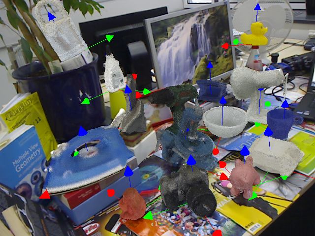
2       Stefan Hinterstoisser et al.

estimate their 3D poses, for manipulation or inspection tasks. Our approach
is based on LINEMOD [1], an efficient method that exploits both depth and
color images to capture the appearance and 3D shape of the object in a set of
templates covering different views of an object. Because the viewpoint of each
template is known, it provides a coarse estimate of the pose of the object when
it is detected.
     However, the initial version of LINEMOD [1] has some disadvantages. First,
templates are learned online, which is difficult to control and results in spotty
coverage of viewpoints. Second, the pose output by LINEMOD is only approx-
imately correct, since a template covers a range of views around its viewpoint.
And finally, the performance of LINEMOD, while extremely good, still suffers
from the presence of false positives.
     In this paper, we show how to overcome these disadvantages, and create a
system based on LINEMOD for the automatic modeling, detection, and tracking
of 3D objects with RGBD sensors. Our main insight is that a 3D model of
the object can be exploited to remedy these deficiencies. Note that accurate
3D models can now be created very quickly [2–5], and requiring a 3D model
beforehand is not a disadvantage anymore. For industrial applications, a detailed
3D model often exists before the real object is even created.
     Given a 3D model of an object, we show how to generate templates that
cover a full view hemisphere by regularly sampling viewpoints of the 3D model.
We also show how the 3D model can be used to obtain a fine estimate of the
object pose, starting from the one provided by the templates. Together with a
simple test based on color, this allows us to remove false positives, by checking if
the object under the recovered pose aligns well with the depth map. Moreover,
we show how to define the templates only with the most useful appearance and
depth information, which allows us to speed up the template detection stage.
The end result is a system that significantly improves the original LINEMOD
implementation in performance, while providing accurate pose for applications.
     In short, we propose a framework that is easy to deploy, reliable, and fast
enough to run in real-time. We also provide a dataset made of 15 registered,
1100+ frame video sequences of 15 various objects for the evaluation of future
competing methods. In the remainder of this paper we first discuss related work,
briefly describe the approach of LINEMOD, introduce our method, represent our
dataset and present an exhaustive evaluation.

2   Related Work
3D object detection and localization is a difficult but important problem with a
long research history. Methods have been developed for detection in photometric
images and range images, and more recently, in registered color/depth images.
We discuss these below.

Camera Images. We can divide image-based object detection into two broad
categories: learning-based and template approaches. Learning-based systems gen-
eralize well to the objects of particular class like human faces [6], cars [7, 8], or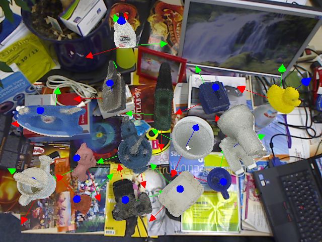
Model Based Training, Detection and Pose Estimation of 3D Objects         3

other objects [9]. Their main limitations are the limited set of object poses they
accept, and the large training database and time. In general, they also do not
return an accurate estimate of the object 3D pose.
    To overcome these limitations, researchers tried to learn the object appear-
ance from 3D models [7, 8, 10]. The approach of Stark et al. [7] relies only on
3D CAD models of cars and Liebelt and Schmid [8] combine geometric shape
and pose priors with natural images. Both of these approaches work well and
also generalize to object classes, but they are not real-time capable, require ex-
pensive training and cannot handle clutter and occlusions well. In [10] authors
use a number of viewpoint-specific shape representations to model the object
category. They rely on contours and introduce a novel feature called BOB (bag
of boundaries), which at a given point in the image is a histogram of bound-
aries from image contours in training images. This feature is later used in the
shape context descriptor for template matching. While it generalizes well, it is
far from real-time and cannot find a precise 3D pose. In contrast, our method
is real-time capable, can learn new objects online from 3D models, can handle
large amount of clutter and moderate occlusions and can detect multiple objects
simultaneously.
    As discussed in [1], template-based approaches [11–14] typically do not re-
quire large training sets or time, as the templates are acquired quickly from views
of the object. However, all these approaches are either susceptible to background
clutter or too slow for real-time performance.

Range Images. Detection of 3D objects in range data has a long history; a
review can be found in [15]. One of the standard approaches for object pose esti-
mation is ICP [16]; however this approach requires an initial estimate and is not
suited for object detection. Approaches based on 3D features are more suitable
and are usually followed by ICP for the pose refinement. Some of these methods
(which assume that a full 3D model is available) include spin-images [17], point
pairs [18, 19], and point-pair histograms [20, 21]. These methods are usually com-
putationally expensive, and have difficulty in scenes with clutter. The method
of Drost et. al [18] can deal with clutter; however, its efficiency and performance
depend directly on the complexity of the 3D scene, which makes it difficult to
use in real-time applications.

RGBD Images. In recent years, a number of methods that rely on RGBD
sensors have been introduced—among them [22] which is subject to object clas-
sification, pose estimation and reconstruction. Similar to us the training data
set is composed of depth and image intensity cues and the object classes are
detected using a modified Hough transform. While being quite effective in real
applications these approaches still require exhaustive training on large data sets.
In [23] Lei et al. study the recognition problem at both the category and the
instance level. In addition they provide a large data set of 3D objects. However,
they have neither demonstrated that their approach work on heavily cluttered
scenes in real time nor that it returns 3D pose as our method does.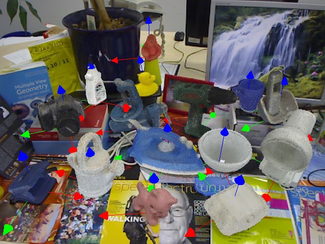
4       Stefan Hinterstoisser et al.

3     Approach
Our approach to object detection is based on LINEMOD [1]. LINEMOD is an
efficient method to detect multi-modal templates in the Kinect output, a depth
map registered to a color image. The LINEMOD templates sample the possible
appearances of the objects to detect, and are built from densely sampled image
gradients and depth map normals. When a template is found, it provides not
only the object’s 2D location in the image, but also a coarse estimate of its pose,
as the templates can easily be labeled with this information.
     In the reminder of the paper, we will show how we generate the templates
automatically from a 3D model with a regular sampling. We also show how
we speed up detection time by keeping only the most useful information in the
templates, how we compute a fine estimate of the object 3D pose, and how we
exploit this pose and the object color to detect outliers.

3.1   Exploiting a 3D Model to Create the Templates
In contrast to online learning approaches [1, 14, 24–26], we build a set of tem-
plates automatically from CAD 3D models. This has several advantages. First,
online learning requires physical interaction of a human operator or a robot with
their environment, and therefore takes time and effort. Furthermore, it usually
takes an educated user and careful manual interaction to collect a well sampled
training set of the object that covers the whole pose range. Online methods usu-
ally follow a greedy approach and they are not guaranteed to lead to optimal
results in terms of trade-off between efficiency and robustness.

3.1.1 Viewpoint Sampling: Viewpoint sampling is crucial in LINEMOD. We
have to balance the trade-off between the coverage of the object for reliability
and the number of template for efficiency. As in [27], we solve this problem by
recursively dividing an icosahedron, the largest convex regular polyhedron. We
substitute each triangle into four almost equilateral triangles, and iterate several
times. As illustrated in Fig. 2, the vertices of the resulting polyhedron give us
then the two out-of-plane rotation angles for the sampled pose with respect to the
coordinate center. In practice we stop at 162 vertices on the upper hemisphere for
a good trade-off. Two adjacent vertices are then approximately 15 degrees apart.
In addition to the these two out of plane rotations, we also created templates
for different in-plane rotations. Furthermore, we generate templates at different
scales by using different sized polyhedrons, using a step size of 10 cm.

3.1.2 Reducing Feature Redundancy: LINEMOD relies on two different
features: color gradients, computed from the color image, and surface normals,
computed from the object 3D model. Both are discretized to a few values by the
algorithm. The color gradients are taken at each image location as the gradient
of largest magnitude over the 3 color channels. The LINEMOD templates are
made from these two features computed densely. We show here that we can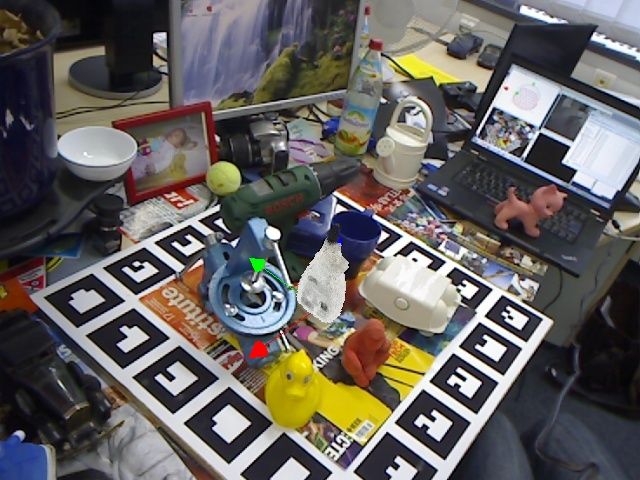
Model Based Training, Detection and Pose Estimation of 3D Objects           5

Fig. 2. Left: Sampling the viewpoints of the upper hemisphere for template generation:
Red vertices represent the virtual camera centers used to generate templates. Note,
that the camera centers are uniformly sampled. Middle: The selected features: Color
gradient features are displayed in red, surface normal features in green. The features
are quasi uniformly spread over the areas where they represent the object best. Right:
15 different texture-less 3D objects used in our experiments.

consider only a subset of the features used in LINEMOD. This speeds up the
detection with no loss of accuracy.

Color Gradient Features: We keep only the main color gradient features
located on the contour of the object silhouette, because we focus on texture-
less objects which exhibit no or only little texture on the interior of the object
silhouette, and because the texture of a given CAD 3D model is not always
available.
    For each sampled pose generated by the method described above, we first
compute the object silhouette by projecting the 3D model under this pose. By
subtracting the eroded silhouette from its original version we quickly obtain the
silhouette contour. We then compute all the color gradients that lie on the silhou-
ette contour and sort them with respect to their magnitudes. This is important
since our silhouette edge is not guaranteed to be only one pixel broad. We then
use a greedy approach where we iterate through this sorted list, starting from the
gradient with the strongest magnitude, and take the first feature that appears
in this list. We then remove from the list the features whose image locations
are close—according to some distance threshold—to the picked feature location,
and we iterate.
    If we have finished iterating through the list of features before a desired
number of features is selected, we decrease the distance threshold by one and
start the process again. The threshold is initially set to the ratio of the area
covered by the silhouette and the number of features that are supposed to be
selected. This heuristic is reasonable since the silhouette contour is usually a one
pixel broad edge such that the initial threshold is simply the maximal possible
distance between two features if these are spread uniformly on an ideal one
pixel broad silhouette. As a result, our efficient method ensures that the selected
features are both robust and, at the same time, almost uniformly spread on the
silhouette (see Fig. 2).

Surface Normal Features: In contrast to color gradient features, we chose
the surface normal features to be selected on the interior of the object silhouette.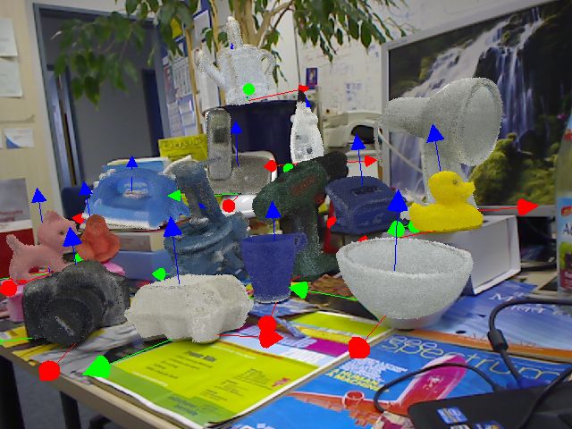
6      Stefan Hinterstoisser et al.

This is because the surface normals on the borders of the projected object are
often not estimated reliably, or not recovered at all.
    As in LINEMOD we discretize the normals computed from the depth map
by considering their orientations. The first difference is that in the case of the
template generation, the depth map is computed from the object 3D model, not
acquired by the Kinect.
    We first remark that normals surrounded by normals of similar orientation
are recovered more reliably. We therefore want to keep these normals during
the creation of the template, and discard the less stable ones. To do so, we first
create a mask for each of the 8 possible values of discretized orientations from
the depth map generated for the object under the considered pose.
    For each of the 8 masks, we then weight each normal with the distance to
the mask boundary. Large distances indicate normals surrounded with normals
of similar orientation. Small distances indicate normals surrounded by different
normals, or normals close to the object silhouette boundaries, and we first di-
rectly reject the normals with a weight smaller than a specific distance—we use
2 in practice.
    However, we can not rely on the weights only to select the normals we want to
keep among the remaining ones. This is because large areas with similar normals
would have a too great influence on the resulting template, and therefore, we
normalize the weights by the size of the mask they belong to.
    We then proceed as for the selection of the color gradients. We first create
a list of the surface normals, ranked according to their normalized weights, and
iteratively select the normals we keep in the final template. It ensures an quasi
uniform spreading of the selected normals (see Fig. 2). Here, the threshold is set
to the square root of the ratio of the area covered by the rendered object and
the number of features we want to keep.

3.2   Postprocessing Detections

For each template detected by LINEMOD—starting with the one with the high-
est similarity score, we first check the consistency of this detection by comparing
the object color with the content of the color image at its location. If it passes
the test, we estimate the 3D pose of the corresponding object. We reject all de-
tections whose 3D pose estimates have not converged properly. Taking the first
n detections that passed all checks, we do a final pose estimate for the best of
them. We use this final estimate in an ultimate depth test for the validity of
the detection. As shown in the results section, these additional tests make our
approach much more reliable than LINEMOD.

3.2.1 Coarse Outlier Removal by Color: Each detected template provides a
coarse estimate of the object pose that is good enough for an efficient check based
on color information. We consider the pixels that lie on the object projection
according to the pose estimate, and count how many of them have the expected
color. We decide a pixel has the expected color if the difference between its hue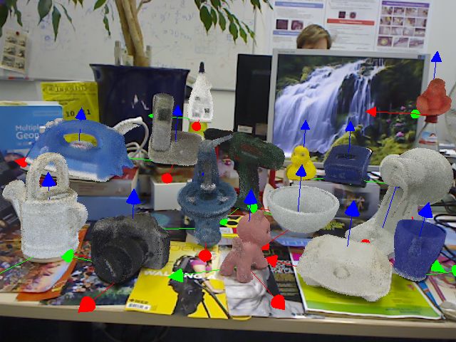
Model Based Training, Detection and Pose Estimation of 3D Objects         7

and the object hue (modulo 2π) is smaller than a threshold—considering the
hue makes the test robust to light changes. If the percentage of pixels that have
their expected color is not large enough (at least 70% in our implementation),
we reject the detection as false positive.
    In practice we do not take into account the pixels that are too close to the
object projection boundaries, to be tolerant to the inaccuracy of the current
pose estimate. This can be done efficiently by eroding the object projection
beforehand.
    We still have to handle black and white objects. Since black and white are not
covered by the hue component, we map them to the hue values of similar colors:
black to blue and white to yellow. This is done by checking the corresponding
saturation and value component before we compute the absolute difference. In
case the value component is below a threshold tv , we set the hue value to blue.
If the value component is larger than tv and the saturation component below a
threshold ts , we set the hue component to yellow. In our case ts = tv = 0.12.

3.2.2 Fast Pose Estimation and Outlier Rejection based on Depth: For
the detections that passed the previous color check, we refine the pose estimate
provided by the template detection. This is performed with the Iterative Closest
Point algorithm to align the 3D model surface with the depth map. The ini-
tial translation is estimated from the depth values covered by the initial model
projection.
    For efficiency, we first subsample the 3D points from the depth map that lie
on the object projection or close to it. To speed up point-to-point matching, we
use the efficient voxel-based ICP method of [28], which relies on a grid that can
be pre-computed for each object. For robustness, at each iteration i, we compute
the alignment using only the inlier 3D points. The inlier points are the ones that
fall within a distance to the 3D model smaller than an adaptive threshold ti .
t0 is initialized to the size of the object, ti+1 is set to three times the average
distance of the inliers to the 3D model at time i. After convergence, if the average
distance of the inliers to the 3D model is too large, we reject the detection as
false positive.
    We repeat this until n = 3 detections passed this check or no detections are
left. Then we perform a slower but finer ICP for the best of these n detections by
considering all the points from the depth map that lie on the object projection
or close to it. The best detection is found by comparing the number of inliers and
their average distance to the 3D model. The final ICP is followed by a final depth
test. For that, we consider the pixels that lie on the object projection according
to the final pose estimate, and count how many of them have the expected depth.
We decide a pixel has the expected depth if the difference between its depth value
and the projected object depth is smaller than a threshold. If the percentage of
pixels that have their expected depth is not large enough (at least 70% in our
implementation), we finally reject the detection as false positive. Otherwise, we
we say that the object was found with the final pose.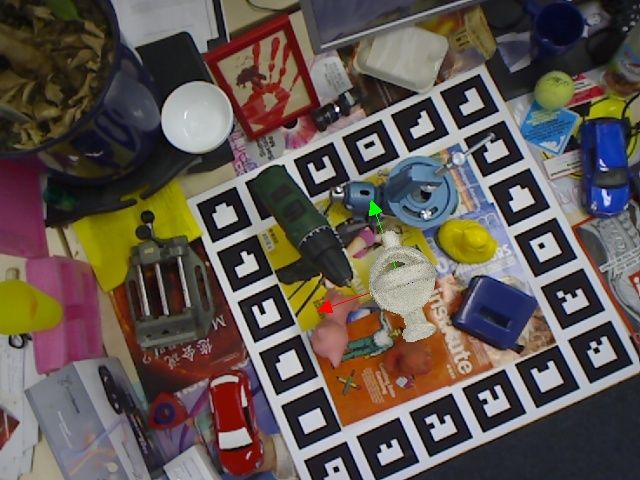
8 Stefan Hinterstoisser et al.
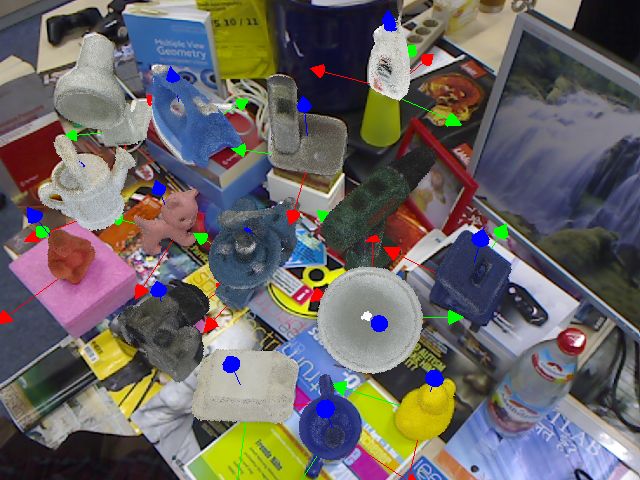
Fig. 3. 15 different texture-less 3D objects are simultaneously detected under different
poses on heavy cluttered background with partial occlusion and illumination changes.
Each detected object is augmented with its 3D model and its coordinate systems.
4 Experiments
For comparison, we created a large dataset of 15 registered video sequences
of 15 texture-less 3D objects. Each object was sticked to the center of a planar
board with markers attached to it, for model and image acquisition. The markers
on the board provided the corresponding ground truth poses. Each object was
reconstructed first using a set of images and the corresponding poses using a
simple voxel based approach. After reconstruction, we added close range and
far range 2D and 3D clutter to the scene and took the evaluation sequences.
Each sequence contains more than 1,100 real images from different view points.
In order to guarantee a well distributed pose space sampling of the dataset
pictures, we uniformly divided the upper hemisphere of the objects into equally
distant pieces and took at most one image per piece. As a result, our sequences
provide uniformly distributed views from 0-360 degree around the object, 0-90
degree tilt rotation, 65 cm-115 cm scaling and ±45 degree in-plane rotation. For
each object, we visualized the cameras color coded with respect to their distance
to the object center in the second column of Figs. 5 and 6.
Since it was already shown in [29] that LINEMOD outperforms DOT [14],
HOG [30], TLD [26] and the method of Steger et al. [13], we compare our method
only to the one of Drost et al. [18]. For [18], we use the binaries kindly provided
by the authors that run on Intel Xeon E5345 processor with 2.33 GHz and 32 GB
RAM. All the other experiments were performed on a standard notebook with
an Intel i7-2820QM processor with 2.3 GHz and 8 GB of RAM. For obtaining
the image and the depth data we used the Primesense(tm) PSDK 5.0 device.
4.1 Robustness
In order to evaluate our approach, we first have to define an appropriate matching
score for a 3D model M: having the ground truth rotation R and translation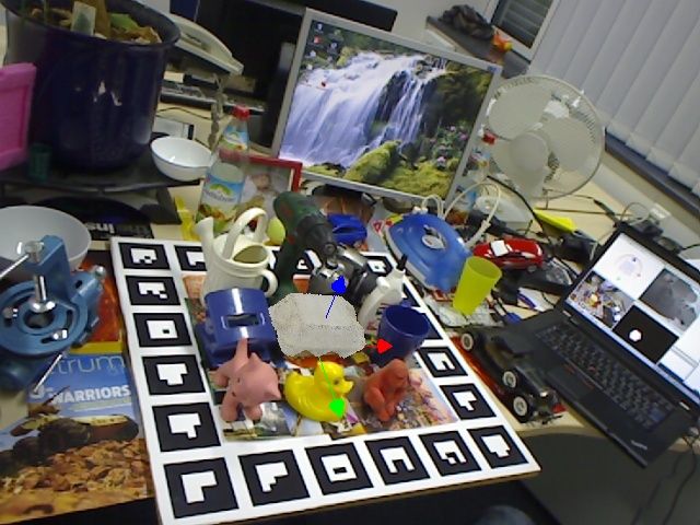
Model Based Training, Detection and Pose Estimation of 3D Objects                                                                                                     9

                              matching score [%]
                                                   95
                                                                                                                        15000

                                                                                                       # of templates
                                                   90
                                                                                                                        10000
                                                   85
                                                                                                                         5000
                                                   80
                                                                                                                              0
                                             rot      5                                       5
                                                   atio 10                                                              rot   5
                                                                                        10        m]                       atio 10                                   5   ]
                                                       n s 15                      15         p [c                             ns                               10 p [cm
                                                          am
                                                             ple 20 25        20          ste                                     am 15 20                   15  ste
                                                                ste                 m ple                                           ple                 20 mple
                                                                                  sa                                                    ste 25              sa
                                                                   p[          le                                                          p[            le
                                                                     deg
                                                                        ]   sca                                                               deg
                                                                                                                                                  ]   sca

               (a)                                                   (b)                                                                     (c)
Fig. 4. Quality of the detections for drilling machine data set with respect to the
viewpoint sampling steps. (a) The matching scores for different numbers of vertices (see
Sec. 3.1). A good trade-off between speed and robustness are 162 vertices for the upper
hemisphere. (b),(c): the matching score decreases if the sample steps increase. We also
display the number of templates with respect to the sampling steps: we made sure that
all necessary poses were covered. A good trade-off between speed and robustness is a
rotation sampling step of 15 degree and a scale sampling step of 10 cm.

Approach         Our Appr. Drost[18] LINEMOD3 LINEMOD1 Our Appr. Drost[18]
Sequence (#pics)               Matching Score                Speed
Ape (1235)        95.8%     86.5%       86.3%    69.4%  127ms      22.7s
Bench Vise (1214) 98.7%     70.7%       98.0%    94.0%  115ms      2.94s
Driller (1187)    93.6%     87.3%       91.8%    81.3%  121ms      2.65s
Cam (1200)        97.5%     78.6%       93.4%    79.5%  148ms      2.81s
Can (1195)        95.4%     80.2%       91.3%    79.5%  122ms      1.60s
Iron (1151)       97.5%     84.9%       95.9%    88.8%  116ms      3.18s
Lamp (1226)       97.7%     93.3%       97.5%    89.8%  125ms      2.29s
Phone (1224)      93.3%     80.7%       88.3%    77.8%  157ms      4.70s
Cat (1178)        99.3%     85.4%       97.9%    88.2%  111ms      7.52s
Hole punch (1236) 95.9%     77.4%       90.5%    78.4%  110ms      8.30s
Duck (1253)       95.9%     46.0%       91.4%    75.9%  104ms      6.97s
Cup (1239)        97.1%     68.4%       87.9%    80.7%  105ms      16.7s
Bowl (1232)       99.9%     95.7%       99.7%    99.5%  97ms       5.18s
Box (1252)        99.8%     97.0%       99.8%    99.1%  101ms      2.94s
Glue (1219)       91.8%     57.2%       80.9%    64.3%  135ms      4.03s
Average (18241)   96.6%     79.3%       92.7%    83.0%  119ms       6.3s

Table 1. Recognition rates for km = 0.1. The first column gives the results of our
method using automatically generated templates (see Sec. 3.1). The second and third
columns give recognition numbers if no postprocessing is performed. For the second
column, we use the best (with respect to the ground truth) out of the first n = 3
detections with the highest similarity score. For the third column, we only evaluate the
detection with the highest similarity score. In the fourth and fifth column, we give the
average runtime of our method and the one of Drost et al. [18] per frame.

T and the estimated rotation R̃ and translation T̃, we compute the average
distance of all model points x from their transformed versions:

                        m = avg k(Rx + T) − (R̃x + T̃)k .                                                                                                                    (1)
                             x∈M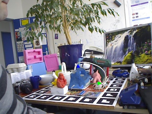
10     Stefan Hinterstoisser et al.

We say that the model was correctly detected and the pose correctly estimated
if km d ≥ m where km is a chosen coefficient and d is the diameter of M. We
still have to define a matching score measure for objects that are ambiguous or
have a subset of views under which they appear to be ambiguous. Such objects
(”cup”,”bowl”,”box” and ”glue”) are shown in Fig. 6. We define the correspond-
ing matching score as:

                  m = avg min k(Rx1 + T) − (R̃x2 + T̃)k .                     (2)
                        x1 ∈M x2 ∈M

Since it was already shown in [29] that LINEMOD outperforms DOT [14],
HOG [30], TLD [26] and the method of Steger et al. [13], we evaluate our new
pipeline with the approach of Drost et al. [18]. This approach – contrary to
the before mentioned ones – does not only perform detection but also pose es-
timation of general 3D objects. For our experiments, we set n = 3 and used
the optimal training parameters as described in Sec. 4.3. As one can see in the
graphs shown in Fig. 5 and 6, our new approach outperforms Drost et al. [18].
    In addition, we compared the output of our new pipeline to the detection
results of LINEMOD. For the latter, we simply used the pose composed by the
rotation under which the detected template was created and the translation
coming from the depth map. Here, we evaluated two strategies: for the first
one, we only took the pose of the detected template whose similarity score was
largest (LINEMOD1). Since our new pipeline evaluates several hypotheses, we
also added curves where we took the best pose with respect to the ground truth
one out of the three best detected templates (LINEMOD3). For both cases, we
can see that our new pipeline drastically increases the recognition performance.
    We also show the matching results for km = 0.1 in Table 1. Matches with
km = 0.1 are also found visually correct. In this table, we see that our new
pipeline outperforms the approach of Drost et al. [18] by average 17.3% and
improves the recognition results by average 13% w.r.t. the original LINEMOD.
    Furthermore, we also evaluated our new approach on the ape, duck and
cup dataset of [1] where we compared our automatically trained LINEMOD
against the manually learned LINEMOD.Our new pipeline obtains almost no
false positves and a superior true positive rate of 98.7% for the cup sequence
(compared to [1]: 96.8%), 98.2% for the ape sequence (compared to [1]: 97.9%)
and 99.5% for the duck sequence (compared to [1]: 97.9).

4.2   Speed

As we see in Tab. 1, our whole recognition pipeline needs in average 119ms to
detect an object in the pose range of 0-360 degree around the object, 0-90 degree
tilt rotation, 65 cm-115 cm scaling and ±45degree in-plane rotation. This is 53
times faster than the approach of Drost et al. and allows real-time recognition.
To cover this pose range we need 3,115 templates. Unoptimized training lasts
from 17 seconds for the ”ape” object to 50 seconds for the ”bench vise” object
and is dependent on the number of vertices to render.
Model Based Training, Detection and Pose Estimation of 3D Objects 11
4.3 Choosing Training Sample Parameters
In order to choose the right parameters for training, we initially took the drill
sequence and evaluated our method with respect to the training parameters. As
we can see in the first graph of Fig. 4, sampling the viewpoints with 162 ver-
tices is a good trade-off between robustness and the number of templates which
have to be matched. The speed performance of our approach is proportional to
this number and thus, using less templates implies shorter runtime. In addition
we made experiments, how the sampling of the scale and the in-plane rotation
influences the robustness and the runtime. As we can see in middle and right
graphs of Fig. 4, a good trade-off is a scale step of 10 cm and a rotation step
of 15 degrees. As we found out, the choice of these parameters gave very good
results for all objects in our database. Therefore, we set them once and for all.
5 Conclusion
We have presented a framework for automatic learning, detection and pose es-
timation of 3D objects using a Kinect. As a first contribution, we showed how
we automatically reduce feature redundancy for color gradients and surface nor-
mals and how we automatically learn templates from a 3D model. For the latter,
we provide a solution of pose space sampling which guarantees a good trade-off
between detection speed and robustness. As a second contribution, we provided
novel means for efficient postprocessing and showed that the pose estimation and
the color information allow us to check the detection hypotheses and to improve
the correct detection rate by 13% with respect to the original LINEMOD. Fur-
thermore, we showed that we significantly outperform the approach of Drost et
al. [18]—a commercial state-of-the-art detection approach that is able to estimate
the object pose. Our final contribution is the proposal of a new dataset made
of 15 registered, 1100+ frame video sequences of 15 various texture-less objects
for the evaluation of future competing methods. The novelty of our sequences
with respect to state-of-the-art datasets is the combination of the following fea-
tures: First, for each sequence and each image, we provide the corresponding 3D
model of the object and its ground truth poses. Second, each sequence uniformly
covers the complete pose space around the registered object. Third, each image
contains heavy close range and far range 2D and 3D clutter.
.
References
1. Hinterstoisser, S., Cagniart, C., Holzer, S., Ilic, S., Konolige, K., Navab, N., Lepetit,
V.: Multimodal Templates for Real-Time Detection of Texture-Less Objects in
Heavily Cluttered Scenes. In: ICCV. (2011)
2. Newcombe, R.A., Izadi, S., Hilliges, O., Molyneaux, D., Kim, D., Davison, A.J.,
Kohli, P., Shotton, J., Hodges, S., Fitzgibbon, A.: KinectFusion: Real-Time Dense
Surface Mapping and Tracking. In: ISMAR. (2011)
3. Pan, Q., Reitmayr, G., Drummond, T.: ProFORMA: Probabilistic Feature-based
On-line Rapid Model Acquisition. In: BMVC. (2009)
4. Weise, T., Wismer, T., Leibe, B., Gool, L.V.: In-hand Scanning with Online Loop
Closure. In: International Workshop on 3-D Digital Imaging and Modeling. (2009)12 Stefan Hinterstoisser et al.
5. Newcombe, R.A., Lovegrove, S.J., Davison, A.J.: DTAM: Dense Tracking and
Mapping in Real-Time. In: ICCV. (2011)
6. Viola, P., Jones, M.: Fast Multi-View Face Detection. In: CVPR. (2003)
7. Stark, M., Goesele, M., Schiele, B.: Back to the Future: Learning Shape Models
from 3D Cad Data. In: BMVC. (2010)
8. Liebelt, J., Schmid, C.: Multi-View Object Class Detection With a 3D Geometric
Model. In: CVPR. (2010)
9. Ferrari, V., Jurie, F., Schmid, C.: From Images to Shape Models for Object De-
tection. IJCV (2009)
10. Payet, N., Todorovic, S.: From contours to 3d object detection and pose estimation.
In: ICCV. (2011) 983–990
11. Gavrila, D., Philomin, V.: Real-Time Object Detection for “smart” Vehicles. In:
ICCV. (1999)
12. Huttenlocher, D., Klanderman, G., Rucklidge, W.: Comparing Images Using the
Hausdorff Distance. TPAMI (1993)
13. Steger, C.: Occlusion Clutter, and Illumination Invariant Object Recognition. In:
International Archives of Photogrammetry and Remote Sensing. (2002)
14. Hinterstoisser, S., Lepetit, V., Ilic, S., Fua, P., Navab, N.: Dominant Orientation
Templates for Real-Time Detection of Texture-Less Objects. In: CVPR. (2010)
15. Mian, A.S., Bennamoun, M., Owens, R.A.: Automatic Correspondence for 3D
Modeling: an Extensive Review. International Journal of Shape Modeling (2005)
16. Zhang, Z.: Iterative Point Matching for Registration of Free-Form Curves. IJCV
(1994)
17. Johnson, A.E., Hebert, M.: Using Spin Images for Efficient Object Recognition in
Cluttered 3 D Scenes. TPAMI (1999)
18. Drost, B., Ulrich, M., Navab, N., Ilic, S.: Model Globally, Match Locally: Efficient
and Robust 3D Object Recognition. In: CVPR. (2010)
19. Mian, A.S., Bennamoun, M., Owens, R.: Three-Dimensional Model-Based Object
Recognition and Segmentation in Cluttered Scenes. TPAMI (2006)
20. Rusu, R.B., Blodow, N., Beetz, M.: Fast Point Feature Histograms (FPFH) for 3D
Registration. In: International Conference on Robotics and Automation. (2009)
21. Tombari, F., Salti, S., Stefano, L.D.: Unique Signatures of Histograms for Local
Surface Description. In: ECCV. (2010)
22. Sun, M., Bradski, G.R., Xu, B.X., Savarese, S.: Depth-Encoded Hough Voting for
Joint Object Detection and Shape Recovery. In: ECCV. (2010)
23. Lai, K., Bo, L., Ren, X., Fox, D.: Sparse distance learning for object recognition
combining rgb and depth information. In: ICRA. (2011) 4007–4013
24. Grabner, M., Grabner., H., Bischof, H.: Learning Features for Tracking. In: CVPR.
(2007)
25. Ozuysal, M., Calonder, M., Lepetit, V., Fua, P.: Fast Keypoint Online Learning
and Recognition. TPAMI (2010)
26. Kalal, Z., Matas, J., Mikolajczyk, K.: P-N Learning: Bootstrapping Binary Clas-
sifiers by Structural Constraints. In: CVPR. (2010)
27. Hinterstoisser, S., Benhimane, S., Lepetit, V., Fua, P., Navab, N.: Simultaneous
Recognition and Homography Extraction of Local Patches With a Simple Linear
Classifier. In: BMVC. (2008)
28. Fitzgibbon, A.: Robust Registration fo 2D and 3D Point Sets. In: BMVC. (2001)
29. Hinterstoisser, S., Ilic, S., Sturm, P., Navab, N., Fua, P., Lepetit, V.: Gradient
Response Maps for Real-Time Detection of Texture-Less Objects. TPAMI (2012)
30. Dalal, N., Triggs, B.: Histograms of Oriented Gradients for Human Detection. In:
CVPR. (2005)Model Based Training, Detection and Pose Estimation of 3D Objects 13
100
matching score [%]
50
Our Method
Drost et al.
LINEMOD1
LINEMOD3
0
8 10 12 14
km [% of object diameter]
100
matching score [%]
50
Our Method
Drost et al.
LINEMOD1
LINEMOD3
0
8 10 12 14
km [% of object diameter]
100
matching score [%]
50
Our Method
Drost et al.
LINEMOD1
LINEMOD3
0
8 10 12 14
km [% of object diameter]
100
matching score [%]
50
Our Method
Drost et al.
LINEMOD1
LINEMOD3
0
8 10 12 14
km [% of object diameter]
matching score [%] 100
50
Our Method
Drost et al.
LINEMOD1
LINEMOD3
0
8 10 12 14
km [% of object diameter]
100
matching score [%]
50
Our Method
Drost et al.
LINEMOD1
LINEMOD3
0
8 10 12 14
km [% of object diameter]
100
matching score [%]
50
Our Method
Drost et al.
LINEMOD1
LINEMOD3
0
8 10 12 14
km [% of object diameter]
Fig. 5. In our experiments, different texture-less 3D objects are detected in real-time
under different poses on heavy cluttered background. Left: Some 3D reconstructed
models. Middle Left: The pose space of the dataset images. The distance of the
cameras to the object is color coded. Middle Right: One test image with the cor-
rectly recognized object. The 3D model of the object is augmented. Right: The
matching scores with respect to different km . The datasets is public available
at http://campar.in.tum.de/twiki/pub/Main/StefanHinterstoisser.14 Stefan Hinterstoisser et al.
100
matching score [%]
50
Our Method
Drost et al.
LINEMOD1
LINEMOD3
0
8 10 12 14
km [% of object diameter]
100
matching score [%]
50
Our Method
Drost et al.
LINEMOD1
LINEMOD3
0
8 10 12 14
km [% of object diameter]
100
matching score [%]
50
Our Method
Drost et al.
LINEMOD1
LINEMOD3
0
8 10 12 14
km [% of object diameter]
100
matching score [%]
50
Our Method
Drost et al.
LINEMOD1
LINEMOD3
0
8 10 12 14
km [% of object diameter]
matching score [%] 100
50
Our Method
Drost et al.
LINEMOD1
LINEMOD3
0
8 10 12 14
km [% of object diameter]
100
matching score [%]
50
Our Method
Drost et al.
LINEMOD1
LINEMOD3
0
8 10 12 14
km [% of object diameter]
100
matching score [%]
50
Our Method
Drost et al.
LINEMOD1
LINEMOD3
0
8 10 12 14
km [% of object diameter]
100
matching score [%]
50
Our Method
Drost et al.
LINEMOD1
LINEMOD3
0
8 10 12 14
km [% of object diameter]
Fig. 6. Another set of 3D objects we used in our exten-
sive experiments. The datasets is public available at
http://campar.in.tum.de/twiki/pub/Main/StefanHinterstoisser.You can also read